New E-Book Release: Math Concepts Everyone Should Know (And Can Learn)

Well, a few weeks ago I broke my toe, which meant that I was forced to sit in my room hour after hour and think about what to do. Luckily, I found something to keep me busy: writing a new math book. The book is called Math Concepts Everyone Should Know (And Can Learn) and was completed yesterday. It is now live on Amazon (click the cover to get to the product page) for the low price of $ 2.99 and can be read without any prior knowledge in mathematics.

I must say that I’m very pleased with the result and I hope you will enjoy the learning experience. The topics are:

– Combinatorics and Probability
– Binomial Distribution
– Banzhaf Power Index
– Trigonometry
– Hypothesis Testing
– Bijective Functions And Infinity

What are Functions? Excerpt from “Math Dialogue: Functions”

T:

What are functions? I could just insert the standard definition here, but I fear that this might not be the best approach for those who have just started their journey into the fascinating world of mathematics. For one, any common textbook will include the definition, so if that’s all you’re looking for, you don’t need to continue reading here. Secondly, it is much more rewarding to build towards the definition step by step. This approach minimizes the risk of developing deficits and falling prey to misunderstandings.

S:

So where do we start?

T:

We have two options here. We could take the intuitive, concept-focused approach or the more abstract, mathematically rigorous path. My recommendation is to go down both roads, starting with the more intuitive approach and taking care of the strict details later on. This will allow you to get familiar with the concept of the function and apply it to solve real-world problems without first delving into sets, Cartesian products as well as relations and their properties.

S:

Sounds reasonable.

T:

Then let’s get started. For now we will think of a function as a mathematical expression that allows us to insert the value of one quantity x and spits out the value of another quantity y. So it’s basically an input-output system.

S:

Can you give me an example of this?

T:

Certainly. Here is a function: y = 2·x + 4. As you can see, there are two variables in there, the so-called independent variable x and the dependent variable y. The variable x is called independent because we are free to choose any value for it. Once a value is chosen, we do what the mathematical expression tells us to do, in this case multiply two by the value we have chosen for x and add four to that. The result of this is the corresponding value of the dependent variable y.

S:

So I can choose any value for x?

T:

That’s right, try out any value.

S:

Okay, I’ll set x = 1 then. When I insert this into the expression I get: y = 2·1 + 4 = 6. What does this tell me?

T:

This calculation tells you that the function y = 2·x + 4 links the input x = 1 with the output y = 6. Go on, try out another input.

S:

Okay, can I use x = 0?

T:

Certainly. Any real number works here.

S:

For x = 0 I get y = 2·0 + 4 = 4. So the function y = 2·x + 4 links the input x = 0 with the output y = 4.

T:

That’s right. Now it should be clear why x is called the independent variable and y the dependent variable. While you may choose any real number for x, sometimes there are common sense restrictions though, we’ll get to that later, the value of y is determined by the form of the function. A few more words on terminology and notation. Sometimes the output is also called the value of the function. We’ve just found that the function y = 2·x + 4 links the input x = 1 with the output y = 6. We could restate that as follows: at x = 1 the function takes on the value y = 6. The other input-output pair we found was x = 0 and y = 4. In other words: at x = 0 the value of the function is y = 4. Keep that in mind.

As for notation, it is very common to use f(x) instead of y. This emphasizes that the expression we are dealing with should be interpreted as a function of the independent variable x. It also allows us to note the input-output pairs in a more compact fashion by including specific values of x in the bracket. Here’s what I mean.

For the function we can write: f(x) = 2·x + 4. Inserting x = 1 we get: f(1) = 2·1 + 4 = 6 or, omitting the calculation, f(1) = 6. The latter is just a very compact way of saying that for x = 1 we get the output y = 6. In a similar manner we can write f(0) = 4 to state that at x = 0 the function takes on the value y = 4. Please insert another value for x using this notation.

S:

Will do. I’ll choose x = -1. Using this value I get: f(-1) = 2·(-1) + 4 = 2 or in short f(-1) = 2. So at x = -1 the value of the function is y = 2. Is all of this correct?

T:

Yes, that’s correct.

S:

You just mentioned that sometimes there are common sense restrictions for the independent variable x. Can I see an example of this?

T:

Okay, let’s get to this right now. Consider the function f(x) = 1/x. Please insert the value x = 1.

S:

For x = 1 I get f(1) = 1/1 = 1. So is it a problem that the output is the same as the input?

T:

Not at all, at x = 1 the function f(x) = 1/x takes on the value y = 1 and this is just fine. The input x = 2 also works well: f(2) = 1/2, so x = 2 is linked with the output y = 1/2. But we will run into problems when trying to insert x = 0.

S:

I see, division by zero. For x = 0 we have f(0) = 1/0 and this expression makes no sense.

T:

That’s right, division by zero is strictly verboten. So whenever an input x would lead to division by zero, we have to rule it out. Let’s state this a bit more elegantly. Every function has a domain. This is just the set of all inputs for which the function produces a real-valued output. For example, the domain of the function f(x) = 2·x + 4 is the set of all real numbers since we can insert any real number x without running into problems. The domain of the function f(x) = 1/x is the set of all real numbers with the number zero excluded since we can use all real numbers as inputs except for zero.

Can you see why the domain of the function f(x) = 1/(3·x – 12) is the set of all real numbers excluding the number four? If it is not obvious, try to insert x = 4.

S:

Okay, for x = 4 I get f(4) = 1/(3·4 – 12) = 1/0. Oh yes, division by zero again.

T:

Correct. That’s why we say that the domain of the function f(x) = 1/(3·x – 12) is the set of all real numbers excluding the number four. Any input x works except for x = 4. So whenever there’s an x somewhere in the denominator, watch out for this. Sometimes we have to exclude inputs for other reasons, too. Consider the function f(x) = sqrt(x). The abbreviation “sqrt” refers to the square root of x. Please compute the value of the function for the inputs x = 0, x = 1 and x = 2.

S:

Will do.

f(0) = sqrt(0) = 0

At x = 0 the value of the function is 0.

f(1) = sqrt(1) = 1

At x = 1 the value of the function is 1.

f(2) = sqrt(2) = 1.4142 …

At x = 2 the value of the function is 1.4142 … All of this looks fine to me. Or is there a problem here?

T:

No problem at all. But now try x = -1.

S:

Okay, f(-1) = sqrt(-1) = … Oh, seems like my calculator spits out an error message here. What’s going on?

T:

Seems like your calculator knows math well. There is no square root of a negative number. Think about it. We say that the square root of the number 4 is 2 because when you multiply 2 by itself you get 4. Note that 4 has another square root and for the same reason. When you multiply -2 by itself, you also get 4, so -2 is also a square root of 4.

Let’s choose another positive number, say 9. The square root of 9 is 3 because when you multiply 3 by itself you get 9. Another square root of 9 is -3 since multiplying -3 by itself leads to 9. So far so good, but what is the square root of -9? Which number can you multiply by itself to produce -9?

S:

Hmmm … 3 doesn’t work since 3 multiplied by itself is 9, -3 also doesn’t work since -3 multiplied by itself is 9. Looks like I can’t think of any number I could multiply by itself to get the result -9.

T:

That’s right, no such real number exists. In other words: there is no real-valued square root of -9. Actually, no negative number has a real-valued square root. That’s why your calculator complained when you gave him the task of finding the square root of -1. For our function f(x) = sqrt(x) all of this means that inserting an x smaller than zero would lead to a nonsensical result. We say that the domain of the function f(x) = sqrt(x) is the set of all positive real numbers including zero.

In summary, when trying to determine the domain of a function, that is, the set of all inputs that lead to a real-valued output, make sure to exclude any values of x that would a) lead to division by zero or b) produce a negative number under a square root sign. Unless faced with a particularly exotic function, the domain of the function is then simply the set of all real numbers excluding values of x that lead to division by zero and those values of x that produce negative numbers under a square root sign.

I promise we will get back to this, but I want to return to the concept of the function before doing some exercises. Let’s go back to the introductory example: f(x) = 2·x + 4. Please make an input-output table for the following inputs: x = -3, -2, -1, 0, 1, 2 and 3.

This was an excerpt from “Math Dialogue: Functions“, available on Amazon for Kindle.

Supernovae – An Introduction

The following is an excerpt from my book “Introduction to Stars: Spectra, Formation, Evolution, Collapse”, available here for Kindle. Enjoy!

A vast number of written recordings show that people watching the night sky on 4 July 1054 had the opportunity to witness the sudden appearance of a new light source in the constellation Taurus that shone four times brighter than our neighbor Venus. The “guest star”, as Chinese astronomers called the mysterious light source, shone so bright that it even remained visible in daylight for over three weeks. After around twenty-one months the guest star disappeared from the night sky, but the mystery remained. What caused the sudden appearance of the light source? Thanks to the steady growth of knowledge and the existence of powerful telescopes, astronomers are now able to answer this question.

The spectacular event of 4 July 1054 was the result of a supernova (plural: supernovae), an enormous explosion that marks the irreversible death of a massive star. Pointing a modern telescope in the direction of the 1054 supernova, one can see a fascinatingly beautiful and still rapidly expanding gas cloud called the Crab Nebula at a distance of roughly 2200 parsecs from Earth. At the center of the Crab Nebula cloud lies a pulsar (Crab Pulsar or PSR B0531+21) having a radius of 10 km and rotating at a frequency of roughly 30 Hz.

Image of the Crab Nebula, taken by the Hubble Space Telescope.

Let’s take a look at the mechanisms that lead to the occurrence of a supernova. At the end of chapter two we noted that a star having an initial mass of eight solar masses or more will form an iron core via a lengthy fusion chain. We might expect that the star could continue its existence by initiating the fusion of iron atoms. But unlike the fusion of lighter elements, the merging of two iron atoms does not produce energy and thus the star cannot fall back on yet another fusion cycle to stabilize itself. Even worse, there are several mechanisms within the core that drain it of much needed energy, the most important being photodisintegration (high-energy photons smash the iron atoms apart) and neutronization (protons and electrons combine to form neutrons). Both of these processes actually speed up the inevitable collapse of the iron core.

Calculations show that the collapse happens at a speed of roughly one-fourth the speed of light, meaning that the core that is initially ten thousand kilometers in diameter will collapse to a neutron star having a radius of only fifteen kilometers in a fraction of a second – literally the blink of an eye. As the core hits the sudden resistance of the degenerate neutrons, the rapid collapse is stopped almost immediately. Because of the high impact speed, the core overshoots its equilibrium position by a bit, springs back, overshoots it again, springs back again, and so on. In short: the core bounces. This process creates massive shock waves that propagate radially outwards, blasting into the outer layers of the star, creating the powerful explosion known as the (collapsing core) supernova.

Within just a few minutes the dying star increases its luminosity to roughly one billion Suns, easily outshining smaller galaxies in the vicinity. It’s no wonder then that this spectacular event can be seen in daylight even without the help of a telescope. The outer layers are explosively ejected with speeds in the order of 50,000 kilometers per second or 30,000 miles per second. As time goes on, the ejected layers slow down and cool off during the expansion and the luminosity of the supernova steadily decreases. Once the envelope has faded into deep space, all that remains of the former star is a compact neutron star or an even more exotic remnant we will discuss in the next section. Supernovas are relatively rare events, it is estimated that they only occur once every fifty years in a galaxy the size of the Milky Way.

At first sight, supernovae may seem like a rather destructive force in the universe. However, this is far from the truth for several reasons, one of which is nucleosynthesis, the creation of elements. Scientists assume that the two lightest elements, hydrogen and helium, were formed during the Big Bang and accordingly, these elements can be found in vast amounts in any part of the universe. Other elements up to iron are formed by cosmic rays (in particular lithium, beryllium and boron) or fusion reactions within a star.

But the creation of elements heavier than iron requires additional mechanisms. Observations indicate that such elements are produced mainly by neutron capture, existing atoms capture a free neutron and transform into a heavier element, either within the envelope of giant stars or supernovae. So supernovae play an important role in providing the universe with many of the heavy elements. Another productive aspect of supernovae is their ability to trigger star formation. When the enormous shock wave emitted from a supernova encounters a giant molecular cloud, it can trigger the collapse of the cloud and thus initiate the formation of a new cluster of stars. Far from destructive indeed.

The rapid collapse of a stellar core is not the only source of supernovae in the universe. A supernova can also occur when a white dwarf locked in a binary system keeps pulling in mass from a partner star. At a critical mass of roughly 1.38 times the mass of the Sun, just slightly below the Chandrasekhar limit, the temperature within the white dwarf would become high enough to re-ignite the carbon. Due to its exotic equilibrium state, the white dwarf cannot make use of the self-regulating mechanism that normally keeps the temperature in check in main sequence stars. The result is thus a runaway fusion reaction that consumes all the carbon and oxygen in the white dwarf within a few seconds and raises the temperature to many billion K, equipping the individual atoms with sufficient kinetic energy to fly off at incredible speeds. This violent explosion lets the remnant glow with around five billion solar luminosities for a very brief time.

Simulation of the runaway nuclear fusion reaction within a white dwarf that became hot enough to re-ignite its carbon content. The result is a violent ejection of its mass.

Stellar Physics – Gaps in the Spectrum

The following is an excerpt from my e-book “Introduction to Stars: Spectra, Formation, Evolution, Collapse” available here for Kindle.

When you look at the spectrum of the heat radiation coming from glowing metal, you will find a continuous spectrum, that is, one that does not have any gaps. You would expect to see the same when looking at light coming from a star. However, there is one significant difference: all stellar spectra have gaps (dark lines) in them. In other words: photons of certain wavelengths seem to be either completely missing or at least arriving in much smaller numbers. Aside from these gaps though, the spectrum is just what you’d expect to see when looking at a heat radiator. So what’s going on here? What can we learn from these gaps?

Spectrum of the Sun. Note the pronounced gaps.

To understand this, we need to delve into atomic physics, or to be more specific, look at how atoms interact with photons. Every atom can only absorb or emit photons of specific wavelengths. Hydrogen atoms for example will absorb photons having the wavelength 4102 A, but do not care about photons having a wavelength 4000 A or 4200 A. Those photons just pass through it without any interaction taking place. Sodium atoms prefer photons with a wavelength 5890 A, when a photon of wavelength 5800 A or 6000 A comes by, the sodium atom is not at all impressed. This is a property you need to keep in mind: every atom absorbs or emits only photons of specific wavelengths.

Suppose a 4102 A photon hits a hydrogen atom. The atom will then absorb the photon, which in crude terms means that the photon “vanishes” and its energy is transferred to one of the atom’s electrons. The electron is now at a higher energy level. However, this state is unstable. After a very short time, the electron returns to a lower energy level and during this process a new photon appears, again having the wavelength 4102 A. So it seems like nothing was gained or lost. Photon comes in, vanishes, electron gains energy, electron loses energy again, photon of same wavelength appears. This seems pointless, why bother mentioning it? Here’s why. The photon that is created when the electron returns to the lower energy level is emitted in a random direction and not the direction the initial photon came from. This is an important point! We can understand the gaps in a spectrum by pondering the consequences of this fact.

Suppose both of us observe a certain heat source. The light from this source reaches me directly while you see the light through a cloud of hydrogen. Both of us are equipped with a device that generates the spectrum of the incoming light. Comparing the resulting spectra, we would see that they are for the most part the same. This is because most photons pass through the hydrogen cloud without any interaction. Consider for example photons of wavelength 5000 A. Hydrogen does not absorb or emit photons of this wavelength, so we will both record the same light intensity at 5000 A. But what about the photons with a 4102 A wavelength?

Imagine a directed stream of these particular photons passing through the hydrogen cloud. As they get absorbed and re-emitted, they get thrown into random directions. Only those photons which do not encounter a hydrogen atom and those which randomly get thrown in your direction will reach your position. Unless the hydrogen cloud is very thin and has a low density, that’s only a very small part of the initial stream. Hence, your spectrum will show a pronounced gap, a line of low light intensity, at λ = 4102 A while in my spectrum no such gap exists.

What if it were a sodium instead of hydrogen cloud? Using the same logic, we can see that now your spectrum should show a gap at λ = 5890 A since this is the characteristic wavelength at which sodium atoms absorb and emit photons. And if it were a mix of hydrogen and sodium, you’d see two dark lines, one at λ = 4102 A due to the presence of hydrogen atoms and another one at λ = 5890 A due to the sodium atoms. Of course, and here comes the fun part, we can reverse this logic. If you record a spectrum and you see gaps at λ = 4102 A and λ = 5890 A, you know for sure that the light must have passed through a gas that contains hydrogen and sodium. So the seemingly unremarkable gaps in a spectrum are actually a neat way of determining what elements sit in a star’s atmosphere! This means that by just looking at a star’s spectrum we can not only determine its temperature, but also its chemical composition at the surface. Here are the results for the Sun:

– Hydrogen 73.5 %

– Helium 24.9 %

– Oxygen 0.8 %

– Carbon 0.3 %

– Iron 0.2 %

– Neon 0.1 %

There are also traces (< 0.1 %) of nitrogen, silicon, magnesium and sulfur. This composition is quite typical for other stars and the universe as a whole: lots of hydrogen (the lightest element), a bit of helium (the second lightest element) and very little of everything else. Mathematical models suggest that even though the interior composition changes significantly over the life time of a star (the reason being fusion, in particular the transformation of hydrogen into helium), its surface composition remains relatively constant in this time.

New Release for Kindle: Introduction to Stars – Spectra, Formation, Evolution, Collapse

I’m happy to announce my new e-book release “Introduction to Stars – Spectra, Formation, Evolution, Collapse” (126 pages, $ 2.99). It contains the basics of how stars are born, what mechanisms power them, how they evolve and why they often die a spectacular death, leaving only a remnant of highly exotic matter. The book also delves into the methods used by astronomers to gather information from the light reaching us through the depth of space. No prior knowledge is required to follow the text and no mathematics beyond the very basics of algebra is used.

If you are interested in learning more, click the cover to get to the Amazon product page:

Here’s the table of contents:

Gathering Information
Introduction
Spectrum and Temperature
Gaps in the Spectrum
Doppler Shift

The Life of a Star
Introduction
Stellar Factories
From Protostar to Star
Main Sequence Stars
Giant Space Onions

The Death of a Star
Introduction
Slicing the Space Onion
Electron Degeneracy
Extreme Matter
Supernovae
Black Holes

Appendix
Answers
Excerpt
Sources and Further Reading

Enjoy the reading experience!

The Placebo Effect – An Overview

There is a major problem with reliance on placebos, like most vitamins and antioxidants. Everyone gets upset about Big Science, Big Pharma, but they love Big Placebo.

– Michael Specter

A Little White Lie

In 1972, Blackwell invited fifty-seven pharmacology students to an hour-long lecture that, unbeknownst to the students, had only one real purpose: bore them. Before the tedious lecture began, the participants were offered a pink or a blue pill and told that the one is a stimulant and the other a sedative (though it was not revealed which color corresponded to which effect – the students had to take their chances). When measuring the alertness of the students later on, the researchers found that 1) the pink pills helped students to stay concentrated and 2) two pills worked better than one. The weird thing about these results: both the pink and blue pills were plain ol’ sugar pills containing no active ingredient whatsoever. From a purely pharmacological point of view, neither pill should have a stimulating or sedative effect. The students were deceived … and yet, those who took the pink pill did a much better job in staying concentrated than those who took the blue pill, outperformed only by those brave individuals who took two of the pink miracle pills. Both the effects of color and number have been reproduced. For example, Luchelli (1972) found that patients with sleeping problems fell asleep faster after taking a blue capsule than after taking an orange one. And red placebos have proven to be more effective pain killers than white, blue or green placebos (Huskisson 1974). As for number, a comprehensive meta-analysis of placebo-controlled trials by Moerman (2002) confirmed that four sugar pills are more beneficial than two. With this we are ready to enter another curious realm of the mind: the placebo effect, where zero is something and two times zero is two times something.

The Oxford Dictionary defines the placebo effect as a beneficial effect produced by a placebo drug or treatment, which cannot be attributed to the properties of the placebo itself and must therefore be due to the patient’s belief in that treatment. In short: mind over matter. The word placebo originates from the Bible (Psalm 116:9, Vulgate version by Jerome) and translates to “I shall please”, which seems to be quite fitting. Until the dawn of modern science, almost all of medicine was, knowingly or unknowingly, based on this effect. Healing spells, astrological rituals, bloodletting … We now know that any improvement in health resulting from such crude treatments can only arise from the fact that the patient’s mind has been sufficiently pleased. Medicine has no doubt come a long way and all of us profit greatly from this. We don’t have to worry about dubious healers drilling holes into our brains to “relieve pressure” (an extremely painful and usually highly ineffective treatment called trepanning), we don’t have to endure the unimaginable pain of a surgeon cutting us open and we live forty years longer than our ancestors. Science has made it possible. However, even in today’s technology-driven world one shouldn’t underestimate the healing powers of the mind.

Before taking a closer look at relevant studies and proposed explanations, we should point out that studying the placebo effect can be a rather tricky affair. It’s not as simple as giving a sugar pill to an ill person and celebrating the resulting improvement in health. All conditions have a certain natural history. Your common cold will build up over several days, peak over the following days and then slowly disappear. Hence, handing a patient a placebo pill (or any other drug for that matter) when the symptoms are at their peak and observing the resulting improvement does not allow you to conclude anything meaningful. In this set-up, separating the effects of the placebo from the natural history of the illness is impossible. To do it right, researchers need one placebo group and one natural history (no-treatment) group. The placebo response is the difference that arises between the two groups. Ignoring natural history is a popular way of “proving” the effectiveness of sham healing rituals and supposed miracle pills. You can literally make any treatment look like a gift from God by knowing the natural history and waiting for the right moment to start the treatment. One can already picture the pamphlet: “93 % of patients were free of symptoms after just three days, so don’t miss out on this revolutionary treatment”. Sounds great, but what they conveniently forget to mention is that the same would have been true had the patients received no treatment.

There are also ethical consideration that need to be taken into account. Suppose you wanted to test how your placebo treatment compares to a drug that is known to be beneficial to a patient’s health. The scientific approach demands setting up one placebo group and one group that receives the well-known drug. How well your placebo treatment performs will be determined by comparing the groups after a predetermined time has passed. However, having one placebo group means that you are depriving people of a treatment that is proven to improve their condition. It goes without saying that this is highly problematic from an ethical point of view. Letting the patient suffer for the quest of knowledge? This approach might be justified if there is sufficient cause to believe that the alternative treatment in question is superior, but this is rarely the case for placebo treatments. While beneficial, their effect is usually much weaker than that of established drugs.

Another source of criticism is the deception of the patient during a placebo treatment. Doctors prefer to be open and honest when discussing a patient’s conditions and the methods of treatment. But a placebo therapy requires them to tell patients that the prescribed pill contains an active ingredient and has proven to be highly effective when in reality it’s nothing but sugar wrapped in a thick layer of good-will. Considering the benefits, we can certainly call it a white lie, but telling it still makes many professionals feel uncomfortable. However, they might be in luck. Several studies have suggested that, surprisingly, the placebo effect still works when the patient is fully aware that he receives placebo pills.

Experimental Evidence

One example of this is the study by Kaptchuk et al. (2010). The Harvard scientists randomly assigned 80 patients suffering from irritable bowel syndrome (IBS) to either a placebo group or no-treatment group. The patients in the placebo group received a placebo pill along with the following explanation: “Placebo pills are made of an inert substance, like sugar pills, and have been shown in clinical studies to produce significant improvement in IBS symptoms through mind-body self-healing processes”. As can be seen from the graph below, the pills did their magic. The improvement in the placebo group was roughly 30 % higher than in the no-treatment group and the low p-value (see appendix for an explanation of the p-value) shows that it is extremely unlikely that this result came to be by chance. Unfortunately, there seems to be a downside to the honesty. Hashish (1988) analyzed the effects of real and sham ultrasound treatment on patients whose impacted lower third molars had been surgically removed and concluded that the effectiveness in producing a placebo response is diminished if the patient comes to understand that the therapy is a placebo treatment rather than the “real” one. So while the placebo-effect does arise even without the element of deception, a fact that is quite astonishing on its own, deception does strengthen the response to the placebo treatment.

Results of Kaptchuk et al. (2010)

Let’s explore some more experimental studies to fully understand the depth and variety of the placebo effect. A large proportion of the relevant research has focused on the effect’s analgesic nature, that is, its ability to reduce pain without impairing consciousness. Amanzio et al. (2001) examined patients who had undergone thoracotomy, a major surgical procedure to gain access to vital organs in the chest and one that is often associated with severe post-operative pain. As handing out sugar pills would have been irresponsible and unethical in this case, the researchers found a more humane method of unearthing the placebo effect: the open-hidden paradigm. All patients received powerful painkillers such as Morphine, Buprenorphine, Tramadol, … However, while one group received the drug in an open manner, administered by a caring clinician in full view of the patient, another group was given the drug in a hidden manner, by means of a computer-programmed drug infusion pump with no clinician present and no indication that the drug was being administered. This set-up enabled the researchers to determine how much of the pain reduction was due to the caring nature of the clinician and the ritual of injecting the drug. The results: the human touch matters and matters a lot. As can be seen from the graph below, every painkiller became significantly more effective when administered in an open fashion. Several follow-on studies (Benedetti et al. 2003, Colloca et al. 2004) confirmed this finding. This demonstrates that the placebo effect goes far beyond the notorious sugar pill, it can also be induced by the caring words of a professional or a dramatic treatment ritual.

Results of Amanzio et al. (2001)

The fact that the human touch is of major importance in any clinical treatment, placebo or otherwise, seems pretty obvious (though its power in reducing pain might have surprised you). Much less obvious are the roles of administration form and treatment ritual, something we shall further explore. For both we can use the following rule of thumb: the more dramatic the intervention, the stronger the placebo response. For example, several studies have shown that an injection with salt-water is more effective in generating the placebo effect than a sugar pill. This is of course despite the fact that both salt-water and sugar pills do not have any direct medical benefits. The key difference lies in the inconveniences associated with the form of delivery: while swallowing a pill takes only a moment and is a rather uncomplicated process, the injection, preparation included, might take up to several minutes and can be quite painful. There’s no doubt that the latter intervention will leave a much stronger impression. Another study (Kaptchuk et al. 2006) came to the exciting conclusion that a nonsensical therapeutic intervention modeled on acupuncture did a significantly better job in reducing arm pain than the sugar pill. While the average pain score in the sham acupuncture group dropped by 0.33 over the course of one week, the corresponding drop in the sugar pill group was only 0.15. Again the more dramatic treatment came out on top.

The experimental results mentioned above might explain why popular ritualistic treatments found in alternative medicine remain so widespread even when there are numerous studies providing ample proof that the interventions lack biological plausibility and produce no direct medical benefits. Despite their scientific shortcomings, such treatments do work. However, this feat is extremely unlikely to be accomplished by strengthening a person’s aura, enhancing life force or harnessing quantum energy, as the brochure might claim. They work mainly (even solely) because of their efficiency in inducing the mind’s own placebo effect. Kaptchuk’s study impressively demonstrates that you can take any arbitrary ritual, back it up with any arbitrary theory to give the procedure pseudo-plausibility and let the placebo effect take over from there. Such a treatment might not be able to compete with cutting-edge drugs, but the benefits will be there. Though one has to wonder about the ethics of providing a patient with a certain treatment when demonstrably a more effective one is available, especially in case of serious diseases.

Don’t Forget Your Lucky Charm

This seems to be a great moment to get in the following entertaining gem. In 2010, Damish et al. invited twenty-eight people to the University of Cologne to take part in a short but sweet experiment that had them play ten balls on a putting green. Half of the participants were given a regular golf ball and managed to get 4.7 putts out of 10 on average. The other half was told they would be playing a “lucky ball” and, sure enough, this increased performance by an astonishing 36 % to 6.4 putts out of 10. I think we can agree that the researchers hadn’t really gotten hold of some magical performance-enhancing “lucky ball” and that the participants most likely didn’t even believe the story of the blessed ball. Yet, the increase was there and the result statistically significant despite the small sample size. So what happened? As you might have expected, this is just another example of the placebo effect (in this particular case also called the lucky charm effect) in action.

OK, so the ball was not really lucky, but it seems that simply floating the far-fetched idea of a lucky ball was enough to put participants into a different mindset, causing them to approach the task at hand in a different manner. One can assume that the story made them less worried about failing and more focused on the game, in which case the marked increase is no surprise at all. Hence, bringing a lucky charm to an exam might not be so superstitious after all. Though we should mention that a lucky charm can only do its magic if the task to be completed requires some skill. If the outcome is completely random, there simply is nothing to gain from being put into a different mindset. So while a lucky charm might be able to help a golfer, student, chess player or even a race car driver, it is completely useless for dice games, betting or winning the lottery.

Let’s look at a few more studies that show just how curious and complex the placebo effect is before moving on to explanations. Shiv et al. (2008) from the Stanford Business School analyzed the economic side of self-healing. They applied electric shocks to 82 participants and then offered them to buy a painkiller (guess that’s also a way to fund your research). The option: get the cheap painkiller for $ 0.10 per pill or the expensive one for $ 2.50 per pill. What the participants weren’t told was that there was no difference between the pills except for the price. Despite that, the price did have an effect on pain reduction. While 61 % of the subjects taking the cheap painkiller reported a significant pain reduction, an impressive 85 % reported the same after treating themselves to the expensive version. The researchers suspect that this is a result of quality expectations. We associate high price with good quality and in case of painkillers good quality equals effective pain reduction. So buying the expensive brand name drug might not be such a bad idea even when there is a chemically identical and lower priced generic drug available. In another study, Shiv et al. also found the same effect for energy drinks. The more expensive energy drink, with price being the only difference, made people report higher alertness and noticeably enhanced their ability to solve word puzzles.

 

This was an excerpt from my Kindle e-book Curiosities of the Mind. To learn more about the placebo effect, as well as other interesting psychological effects such as the chameleon effect, Mozart effect and the actor-observer bias, click here. (Link to Amazon.com)

The Mozart Effect – Hype and Reality

The idea that music can make you smarter became very popular in the mid-nineties under the name “Mozart effect” and has remained popular ever since. The hype began with the publication of Rauscher et al. (1993) in the journal Nature. The researchers discovered that participants who were exposed to the aforementioned Mozart sonata performed better on the Stanford-Binet IQ test than those who listened to verbal relaxation instructions or sat in silence.

This revelation caused armies of mothers and fathers to storm the CD stores and bombard their children with Mozart music. One US governor ordered the distribution of Mozart CD’s by hospitals to all mothers following the birth of a child. Not surprisingly, marketers eagerly joined the fun (with increasingly ridiculous claims about the effect of music on intelligence) to profit from the newly-found “get-smart-quick” scheme. What got lost in the hype however was the fact that Rauscher et al. never found or claimed that exposure to Mozart would increase your IQ in general. Neither did they claim that the performance on an IQ test is a reliable indicator of how smart a person is. All they demonstrated was that exposure to an enjoyable musical piece led to a temporary (< 15 minutes) increase in spatial reasoning ability, not more, not less. Despite that, the study suffered the fate all studies are bound to suffer when they fall into the hands of the tabloid media, politicians and marketers: the results get distorted and blown out of proportion.

By the way: I wonder if mothers and fathers would have been just as eager to expose their children to Mozart had they known about some of the less flattering pieces written by the brilliant composer, among them the canon in B-flat major titled “Leck mich im Arsch” (which translates to “Kiss my Ass”) and the scatological canon “Bona Nox!” which includes the rather unsophisticated line “shit in your bed and make it burst”. These are just two examples of the many obscene and sometimes even pornographic pieces the party animal Mozart wrote for boozy nights with his friends. One can picture the young composer and his companions sitting in a flat in Vienna singing obscene songs after downing a few bottles of wine while concerned mothers cover their children’s ears, cursing the young generation and their vile music. That’s the side of Mozart you won’t get to hear in orchestral concerts.

But back to the topic. So whatever happened to the Mozart effect? Hype aside, is there anything to it? The thorough 1999 meta-analysis of Mozart effect studies by Chabris came to the conclusion that the popularized version of the effect is most certainly incorrect. Listening to Mozart, while no doubt a very enjoyable and stimulating experience, does not permanently raise your IQ or make you more intelligent. However, said meta analysis, as well as the 2002 Husain et al. study described above, did find a small cognitive enhancement resulting from exposure to Mozart’s sonata. The explanation of the enhancement turned out to be somewhat sobering though.

In the original study, Rauscher et al. proposed that Mozart’s music is able to prime spatial abilities in a direct manner because of similarities in neural activation. Further discussion and experiments showed that such a direct link is rather unlikely though, especially in light of the results of Nantais and Schellenberg (1999). In this study participants performed a spatial reasoning task after either listening to Mozart’s sonata or hearing a narrated story. When the reasoning task was completed, the participants were asked which of the two, Mozart’s piece or the story, they preferred. The result: participants who preferred the sonata performed better on the spatial reasoning task after listening to the piece and participants who preferred the story performed better on the test after hearing the story. However, participants who listened to Mozart’s music and stated that they would have preferred the story instead did not show the cognitive improvement. Overall the researchers found no benefit in the Mozart condition. All of the above implies that the enhancement in performance is a result of exposure to a preferred stimulus rather than a direct link between Mozart and cognition. It seems that the Mozart effect is just a small part of a broader psychological phenomenon that goes a little something like this: experiencing a preferred stimulus, be it a musical piece, a narrated story or a funny comic book, has a positive effect on arousal and mood and this in turn enhances cognitive abilities.

This was an extract from my Kindle e-book Curiosities of the Mind. Check it out if you interested in learning more about the psychological effects of music as well as other common psychological effects such as the false consensus bias, the placebo effect, the chameleon effect, …

The Weirdness of Empty Space – Casimir Force

(This is an excerpt from The Book of Forces – enjoy!)

The forces we have discussed so far are well-understood by the scientific community and are commonly featured in introductory as well as advanced physics books. In this section we will turn to a more exotic and mysterious interaction: the Casimir force. After a series of complex quantum mechanical calculations, the Dutch physicist Hendrick Casimir predicted its existence in 1948. However, detecting the interaction proved to be an enormous challenge as this required sensors capable picking up forces in the order of 10^(-15) N and smaller. It wasn’t until 1996 that this technology became available and the existence of the Casimir force was experimentally confirmed.

So what does the Casimir force do? When you place an uncharged, conducting plate at a small distance to an identical plate, the Casimir force will pull them towards each other. The term “conductive” refers to the ability of a material to conduct electricity. For the force it plays no role though whether the plates are actually transporting electricity in a given moment or not, what counts is their ability to do so.

The existence of the force can only be explained via quantum theory. Classical physics considers the vacuum to be empty – no particles, no waves, no forces, just absolute nothingness. However, with the rise of quantum mechanics, scientists realized that this is just a crude approximation of reality. The vacuum is actually filled with an ocean of so-called virtual particles (don’t let the name fool you, they are real). These particles are constantly produced in pairs and annihilate after a very short period of time. Each particle carries a certain amount of energy that depends on its wavelength: the lower the wavelength, the higher the energy of the particle. In theory, there’s no upper limit for the energy such a particle can have when spontaneously coming into existence.

So how does this relate to the Casimir force? The two conducting plates define a boundary in space. They separate the space of finite extension between the plates from the (for all practical purposes) infinite space outside them. Only particles with wavelengths that are a multiple of the distance between the plates fit in the finite space, meaning that the particle density (and thus energy density) in the space between the plates is smaller than the energy density in the pure vacuum surrounding them. This imbalance in energy density gives rise to the Casimir force. In informal terms, the Casimir force is the push of the energy-rich vacuum on the energy-deficient space between the plates.

(Illustration of Casimir force)

It gets even more puzzling though. The nature of the Casimir force depends on the geometry of the plates. If you replace the flat plates by hemispherical shells, the Casimir force suddenly becomes repulsive, meaning that this specific geometry somehow manages to increase the energy density of the enclosed vacuum. Now the even more energy-rich finite space pushes on the surrounding infinite vacuum. Trippy, huh? So which shapes lead to attraction and which lead to repulsion? Unfortunately, there is no intuitive way to decide. Only abstract mathematical calculations and sophisticated experiments can provide an answer.

We can use the following formula to calculate the magnitude of the attractive Casimir force FCS between two flat plates. Its value depends solely on the distance d (in m) between the plates and the area A (in m²) of one plate. The letters h = 6.63·10^(-34) m² kg/s and c = 3.00·10^8 m/s represent Plank’s constant and the speed of light.

FCS = π·h·c·A / (480·d^4) ≈ 1.3·10^(-27)·A / d^4

(The sign ^ stands for “to the power”) Note that because of the exponent, the strength of the force goes down very rapidly with increasing distance. If you double the size of the gap between the plates, the magnitude of the force reduces to 1/2^4 = 1/16 of its original value. And if you triple the distance, it goes down to 1/3^4 = 1/81 of its original value. This strong dependence on distance and the presence of Plank’s constant as a factor cause the Casimir force to be extremely weak in most real-world situations.

————————————-

Example 24:

a) Calculate the magnitude of the Casimir force experienced by two conducting plates having an area A = 1 m² each and distance d = 0.001 m (one millimeter). Compare this to their mutual gravitational attraction given the mass m = 5 kg of one plate.

b) How close do the plates need to be for the Casimir force to be in the order of unity? Set FCS = 1 N.

Solution:

a)

Inserting the given values into the formula for the Casimir force leads to (units not included):

FCS = 1.3·10^(-27)·A/d^4
FCS = 1.3·10^(-27) · 1 / 0.0014
FCS ≈ 1.3·10^(-15) N

Their gravitational attraction is:

FG = G·m·M / r²
FG = 6.67·10^(-11)·5·5 / 0.001²
FG ≈ 0.0017 N

This is more than a trillion times the magnitude of the Casimir force – no wonder this exotic force went undetected for so long.  I should mention though that the gravitational force calculated above should only be regarded as a rough approximation as Newton’s law of gravitation is tailored to two attracting spheres, not two attracting plates.

b)

Setting up an equation we get:

FCS = 1.3·10^(-27)·A/d^4
1 = 1.3·10^(-27) · 1 / d^4

Multiply by d4:

d4 = 1.3·10^(-27)

And apply the fourth root:

d ≈ 2·10^(-7) m = 200 nanometers

This is roughly the size of a common virus and just a bit longer than the wavelength of violet light.

————————————-

The existence of the Casimir force provides an impressive proof that the abstract mathematics of quantum mechanics is able to accurately describe the workings of the small-scale universe. However, many open questions remain. Quantum theory predicts the energy density of the vacuum to be infinitely large. According to Einstein’s theory of gravitation, such a concentration of energy would produce an infinite space-time curvature and if this were the case, we wouldn’t exist. So either we don’t exist (which I’m pretty sure is not the case) or the most powerful theories in physics are at odds when it comes to the vacuum.

All about the Gravitational Force (For Beginners)

(This is an excerpt from The Book of Forces)

All objects exert a gravitational pull on all other objects. The Earth pulls you towards its center and you pull the Earth towards your center. Your car pulls you towards its center and you pull your car towards your center (of course in this case the forces involved are much smaller, but they are there). It is this force that invisibly tethers the Moon to Earth, the Earth to the Sun, the Sun to the Milky Way Galaxy and the Milky Way Galaxy to its local galaxy cluster.

Experiments have shown that the magnitude of the gravitational attraction between two bodies depends on their masses. If you double the mass of one of the bodies, the gravitational force doubles as well. The force also depends on the distance between the bodies. More distance means less gravitational pull. To be specific, the gravitational force obeys an inverse-square law. If you double the distance, the pull reduces to 1/2² = 1/4 of its original value. If you triple the distance, it goes down to 1/3² = 1/9 of its original value. And so on. These dependencies can be summarized in this neat formula:

F = G·m·M / r²

With F being the gravitational force in Newtons, m and M the masses of the two bodies in kilograms, r the center-to-center distance between the bodies in meters and G = 6.67·10^(-11) N m² kg^(-2) the (somewhat cumbersome) gravitational constant. With this great formula, that has first been derived at the end of the seventeenth century and has sparked an ugly plagiarism dispute between Newton and Hooke, you can calculate the gravitational pull between two objects for any situation.

(Gravitational attraction between two spherical masses)

If you have trouble applying the formula on your own or just want to play around with it a bit, check out the free web applet Newton’s Law of Gravity Calculator that can be found on the website of the UNL astronomy education group. It allows you to set the required inputs (the masses and the center-to-center distance) using sliders that are marked special values such as Earth’s mass or the distance Earth-Moon and calculates the gravitational force for you.

————————————-

Example 3:

Calculate the gravitational force a person of mass m = 72 kg experiences at the surface of Earth. The mass of Earth is M = 5.97·10^24 kg (the sign ^ stands for “to the power”) and the distance from the center to the surface r = 6,370,000 m. Using this, show that the acceleration the person experiences in free fall is roughly 10 m/s².

Solution:

To arrive at the answer, we simply insert all the given inputs into the formula for calculating gravitational force.

F = G·m·M / r²
F = 6.67·10^(-11)·72·5.97·10^24 / 6,370,000² N ≈ 707 N

So the magnitude of the gravitational force experienced by the m = 72 kg person is 707 N. In free fall, he or she is driven by this net force (assuming that we can neglect air resistance). Using Newton’s second law we get the following value for the free fall acceleration:

F = m·a
707 N = 72 kg · a

Divide both sides by 72 kg:

a = 707 / 72 m/s² ≈ 9.82 m/s²

Which is roughly (and more exact than) the 10 m/s² we’ve been using in the introduction. Except for the overly small and large numbers involved, calculating gravitational pull is actually quite straight-forward.

As mentioned before, gravitation is not a one-way street. As the Earth pulls on the person, the person pulls on the Earth with the same force (707 N). However, Earth’s mass is considerably larger and hence the acceleration it experiences much smaller. Using Newton’s second law again and the value M = 5.97·1024 kg for the mass of Earth we get:

F = m·a
707 N = 5.97·10^24 kg · a

Divide both sides by 5.97·10^24 kg:

a = 707 / (5.97·10^24) m/s² ≈ 1.18·10^(-22) m/s²

So indeed the acceleration the Earth experiences as a result of the gravitational attraction to the person is tiny.

————————————-

Example 4:

By how much does the gravitational pull change when the  person of mass m = 72 kg is in a plane (altitude 10 km = 10,000 m) instead of the surface of Earth? For the mass and radius of Earth, use the values from the previous example.

Solution:

In this case the center-to-center distance r between the bodies is a bit larger. To be specific, it is the sum of the radius of Earth 6,370,000 m and the height above the surface 10,000 m:

r = 6,370,000 m + 10,000 m = 6,380,000 m

Again we insert everything:

F = G·m·M / r²
F = 6.67·10^(-11)·72·5.97·10^24 / 6,380,000² N ≈ 705 N

So the gravitational force does not change by much (only by 0.3 %) when in a plane. 10 km altitude are not much by gravity’s standards, the height above the surface needs to be much larger for a noticeable difference to occur.

————————————-

With the gravitational law we can easily show that the gravitational acceleration experienced by an object in free fall does not depend on its mass. All objects are subject to the same 10 m/s² acceleration near the surface of Earth. Suppose we denote the mass of an object by m and the mass of Earth by M. The center-to-center distance between the two is r, the radius of Earth. We can then insert all these values into our formula to find the value of the gravitational force:

F = G·m·M / r²

Once calculated, we can turn to Newton’s second law to find the acceleration a the object experiences in free fall. Using F = m·a and dividing both sides by m we find that:

a = F / m = G·M / r²

So the gravitational acceleration indeed depends only on the mass and radius of Earth, but not the object’s mass. In free fall, a feather is subject to the same 10 m/s² acceleration as a stone. But wait, doesn’t that contradict our experience? Doesn’t a stone fall much faster than a feather? It sure does, but this is only due to the presence of air resistance. Initially, both are accelerated at the same rate. But while the stone hardly feels the effects of air resistance, the feather is almost immediately slowed down by the collisions with air molecules. If you dropped both in a vacuum tube, where no air resistance can build up, the stone and the feather would reach the ground at the same time! Check out an online video that shows this interesting vacuum tube experiment, it is quite enlightening to see a feather literally drop like a stone.

(All bodies are subject to the same gravitational acceleration)

Since all objects experience the same acceleration near the surface of Earth and since this is where the everyday action takes place, it pays to have a simplified equation at hand for this special case. Denoting the gravitational acceleration by g (with g ≈ 10 m/s²) as is commonly done, we can calculate the gravitational force, also called weight, an object of mass m is subject to at the surface of Earth by:

F = m·g

So it’s as simple as multiplying the mass by ten. Depending on the application, you can also use the more accurate factor g ≈ 9.82 m/s² (which I will not do in this book). Up to now we’ve only been dealing with gravitation near the surface of Earth, but of course the formula allows us to compute the gravitational force and acceleration near any other celestial body. I will spare you trouble of looking up the relevant data and do the tedious calculations for you. In the table below you can see what gravitational force and acceleration a person of mass m = 72 kg would experience at the surface of various celestial objects. The acceleration is listed in g’s, with 1 g being equal to the free-fall acceleration experienced near the surface of Earth.

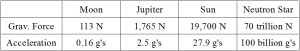
So while jumping on the Moon would feel like slow motion (the free-fall acceleration experienced is comparable to what you feel when stepping on the gas pedal in a common car), you could hardly stand upright on Jupiter as your muscles would have to support more than twice your weight. Imagine that! On the Sun it would be even worse. Assuming you find a way not get instantly killed by the hellish thermonuclear inferno, the enormous gravitational force would feel like having a car on top of you. And unlike temperature or pressure, shielding yourself against gravity is not possible.

What about the final entry? What is a neutron star and why does it have such a mind-blowing gravitational pull? A neutron star is the remnant of a massive star that has burned its fuel and exploded in a supernova, no doubt the most spectacular light-show in the universe. Such remnants are extremely dense – the mass of several suns compressed into an almost perfect sphere of just 20 km radius. With the mass being so large and the distance from the surface to the center so small, the gravitational force on the surface is gigantic and not survivable under any circumstances.

If you approached a neutron star, the gravitational pull would actually kill you long before reaching the surface in a process called spaghettification. This unusual term, made popular by the brilliant physicist Stephen Hawking, refers to the fact that in intense gravitational fields objects are vertically stretched and horizontally compressed. The explanation is rather straight-forward: since the strength of the gravitational force depends on the distance to the source of said force, one side of the approaching object, the side closer to the source, will experience a stronger pull than the opposite side. This leads to a net force stretching the object. If the gravitational force is large enough, this would make any object look like a thin spaghetti. For humans spaghettification would be lethal as the stretching would cause the body to break apart at the weakest spot (which presumably is just above the hips). So my pro-tip is to keep a polite distance from neutron stars.

Antimatter Production – Present and Future

When it comes to using antimatter for propulsion, getting sufficient amounts of the exotic fuel is the biggest challenge. For flights within the solar system, hybrid concepts would require several micrograms of antimatter, while pure antimatter rockets would consume dozens of kilograms per trip. And going beyond the solar system would demand the production of several metric tons and more.

We are very, very far from this. Currently around 10 nanograms of anti-protons are produced in the large particles accelerators each year. At this rate it would take 100 years to produce one measly microgram and 100 billion years to accumulate one kilogram. However, the antimatter production rate has seen exponential growth, going up by sixteen orders of magnitude over the past decades, and this general trend will probably continue for some time.

Even with a noticeable slowdown in this exponential growth, gram amounts of anti-protons could be manufactured each year towards the end of the 21st century, making hybrid antimatter propulsion feasible. With no slowdown, the rate could even reach kilograms per year by then. While most physicists view this as an overly optimistic estimate, it is not impossible considering the current trend in antimatter production and the historic growth of liquid hydrogen and uranium production rates (both considered difficult to manufacture in the past).

There is still much to be optimized in the production of antimatter. The energy efficiency at present is only 10-9, meaning that you have to put in one gigajoule of pricey electric energy to produce a single joule of antimatter energy. The resulting costs are a staggering 62.5 trillion USD per gram of anti-protons, making antimatter the most expensive material known to man. So if you want to tell your wife how precious she is to you (and want to get rid of her at the same time), how about buying her a nice anti-matter scarf?

Establishing facilities solely dedicated to antimatter production, as opposed to the by-product manufacturing in modern particle accelerators, would significantly improve the situation. NASA experts estimate that an investment of around 5 billion USD is sufficient to build such a first generation antimatter factory. This step could bring the costs of anti-protons down to 25 billion USD per gram and increase the production rate to micrograms per year.

While we might not see kilogram amounts of antimatter or antimatter propulsion systems in our lifetime, the production trend over the next few decades will reveal much about the feasibility of antimatter rockets and interstellar travel. If the optimists are correct, and that’s a big if, the grandchildren of our grandchildren’s grandchildren might watch the launch of the first spacecraft capable of reaching neighboring stars. Sci-fi? I’m sure that’s what people said about the Moon landing and close-up pictures from Mars and Jupiter just a lifetime ago.

For more information, check out my ebook Antimatter Propulsion.

New Release for Kindle: Antimatter Propulsion

I’m very excited to announce the release of my latest ebook called “Antimatter Propulsion”. I’ve been working working on it like a madman for the past few months, going through scientific papers and wrestling with the jargon and equations. But I’m quite satisfied with the result. Here’s the blurb, the table of contents and the link to the product page. No prior knowledge is required to enjoy the book.

Many popular science fiction movies and novels feature antimatter propulsion systems, from the classic Star Trek series all the way to Cameron’s hit movie Avatar. But what exactly is antimatter? And how can it be used accelerate rockets? This book is a gentle introduction to the science behind antimatter propulsion. The first section deals with antimatter in general, detailing its discovery, behavior, production and storage. This is followed by an introduction to propulsion, including a look at the most important quantities involved and the propulsion systems in use or in development today. Finally, the most promising antimatter propulsion and rocket concepts are presented and their feasibility discussed, from the solid core concept to antimatter initiated microfusion engines, from the Valkyrie project to Penn State’s AIMStar spacecraft.

Section 1: Antimatter

The Atom
Dirac’s Idea
Anti-Everything
An Explosive Mix
Proton and Anti-Proton Annihilation
Sources of Antimatter
Storing Antimatter
Getting the Fuel

Section 2: Propulsion Basics

Conservation of Momentum
♪ Throw, Throw, Throw Your Boat ♫
So What’s The Deal?
May The Thrust Be With You
Acceleration
Specific Impulse and Fuel Requirements
Chemical Propulsion
Electric Propulsion
Fusion Propulsion

Section 3: Antimatter Propulsion Concepts

Solid Core Concept
Plasma Core Concept
Beamed Core Concept
Antimatter Catalyzed Micro-Fission / Fusion
Antimatter Initiated Micro-Fusion

Section 4: Antimatter Rocket Concepts

Project Valkyrie
ICAN-II
AIMStar
Dust Shields

You can purchase “Antimatter Propulsion” here for $ 2.99.

New Release for Kindle: Math Shorts – Derivatives

The rich and exciting field of calculus begins with the study of derivatives. This book is a practical introduction to derivatives, filled with down-to-earth explanations, detailed examples and lots of exercises (solutions included). It takes you from the basic functions all the way to advanced differentiation rules and proofs. Check out the sample for the table of contents and a taste of the action. From the author of “Mathematical Shenanigans”, “Great Formulas Explained” and the “Math Shorts” series. A supplement to this book is available under the title “Exercises to Math Shorts – Derivatives”. It contains an additional 28 exercises including detailed solutions.

Note: Except for the very basics of algebra, no prior knowledge is required to enjoy this book.

Table of Contents:

– Section 1: The Big Picture

– Section 2: Basic Functions and Rules

Power Functions
Sum Rule and Polynomial Functions
Exponential Functions
Logarithmic Functions
Trigonometric Functions

– Section 3: Advanced Differentiation Rules

I Know That I Know Nothing
Product Rule
Quotient Rule
Chain Rule

– Section 4: Limit Definition and Proofs

The Formula
Power Functions
Constant Factor Rule and Sum Rule
Product Rule

– Section 5: Appendix

Solutions to the Problems
Copyright and Disclaimer
Request to the Reader

Differential Equations – The Big Picture

Population Growth

So you want to learn about differential equations? Excellent choice. Differential equations are not only of central importance to science, they can also be quite stimulating and fun (that’s right). In the broadest sense, a differential equation is any equation that connects a function with one or more of its derivatives. What makes these kinds of equations particularly important?

Remember that a derivative expresses the rate of change of a quantity. So the differential equation basically establishes a link between the rate of change of said quantity and its current value. Such a link is very common in nature. Consider population growth. It is obvious that the rate of change will depend on the current size of the population. The more animals there are, the more births (and deaths) we can expect and hence the faster the size of the population will change.

A commonly used model for population growth is the exponential model. It is based on the assumption that the rate of change is proportional to the current size of the population. Let’s put this into mathematical form. We will denote the size of the population by N (measured in number of animals) and the first derivative with respect to time by dN/dt (measured in number of animals per unit time). Note that other symbols often used for the first derivative are N’ and Ṅ. We will however stick to the so-called Leibniz notation dN/dt as it will prove to be quite instructive when dealing with separable differential equations. That said, let’s go back to the exponential model.

With N being the size of the population and dN/dt the corresponding rate of change, our assumption of proportionality between the two looks like this:

with r being a constant. We can interpret r as the growth rate. If r > 0, then the population will grow, if r < 0, it will shrink. This model has proven to be successful for relatively small animal populations. However, there’s one big flaw: there is no limiting value. According to the model, the population would just keep on growing and growing until it consumes the entire universe. Obviously and luckily, bacteria in Petri dish don’t behave this way. For a more accurate model, we need to take into account the limits of the environment.

The differential equation that forms the basis of the logistic model, called Verhulst equation in honor of the Belgian mathematician Pierre François Verhulst, does just that. Just like the differential equation for exponential growth, it relates the current size N of the population to its rate of change dN/dt, but also takes into account the finite capacity K of the environment:

Take a careful look at the equation. Even without any calculations a differential equation can tell a vivid story. Suppose for example that the population is very small. In this case N is much smaller than K, so the ratio N/K is close to zero. This means that we are back to the exponential model. Hence, the logistic model contains the exponential model as a special case. Great! The other extreme is N = K, that is, when the size of the population reaches the capacity. In this case the ratio N/K is one and the rate of change dN/dt becomes zero, which is exactly what we were expecting. No more growth at the capacity.

Definition and Equation of Motion

Now that you have seen two examples of differential equations, let’s generalize the whole thing. For starters, note that we can rewrite the two equations as such:

Denoting the dependent variable with x (instead of N) and higher order derivatives with dnx/dtn (with n = 2 resulting in the second derivative, n = 3 in the third derivative, and so on), the general form of a differential equation looks like this:

Wow, that looks horrible! But don’t worry. We just stated in the broadest way possible that a differential equation is any equation that connects a function x(t) with one or more its derivatives dx/dt, d2x/dt2, and so on. The above differential equation is said to have the order n. Up to now, we’ve only been dealing with first order differential equations.

The following equation is an example of a second order differential equation that you’ll frequently come across in physics. Its solution x(t) describes the position or angle over time of an oscillating object (spring, pendulum).

with c being a constant. Second order differential equations often arise naturally from Newton’s equation of motion. This law, which even the most ruthless crook will never be able to break, states that the object’s mass m times the acceleration a experienced by it is equal to the applied net force F:

The force can be a function of the object’s location x (spring), the velocity v = dx/dt (air resistance), the acceleration a = d2x/dt2 (Bremsstrahlung) and time t (motor):

Hence the equation of motion becomes:

A second order differential equation which leads to the object’s position over time x(t) given the forces involved in shaping its motion. It might not look pretty to some (it does to me), but there’s no doubt that it is extremely powerful and useful.

Equilibrium Points

To demonstrate what equilibrium points are and how to compute them, let’s take the logistic model a step further. In the absence of predators, we can assume the fish in a certain lake to grow according to Verhulst’s equation. The presence of fishermen obviously changes the dynamics of the population. Every time a fisherman goes out, he will remove some of the fish from the population. It is safe to assume that the success of the fisherman depends on the current size of the population: the more fish there are, the more he will be able to catch. We can set up a modified version of Verhulst’s equation to describe the situation mathematically:

with a constant c > 0 that depends on the total number of fishermen, the frequency and duration of their fishing trips, the size of their nets, and so on. Solving this differential equation is quite difficult. However, what we can do with relative ease is finding equilibrium points.

Remember that dN/dt describes the rate of change of the population. Hence, by setting dN/dt = 0, we can find out if and when the population reaches a constant size. Let’s do this for the above equation.

This leads to two solutions:

The first equilibrium point is quite boring. Once the population reaches zero, it will remain there. You don’t need to do math to see that. However, the second equilibrium point is much more interesting. It tells us how to calculate the size of the population in the long run from the constants. We can also see that a stable population is only possible if c < r.

Note that not all equilibrium points that we find during such an analysis are actually stable (in the sense that the system will return to the equilibrium point after a small disturbance). The easiest way to find out whether an equilibrium point is stable or not is to plot the rate of change, in this case dN/dt, over the dependent variable, in this case N. If the curve goes from positive to negative values at the equilibrium point, the equilibrium is stable, otherwise it is unstable.

(This was an excerpt from my e-book “Math Shorts – Introduction to Differential Equations”)

Modeling Theme Park Queues

Who doesn’t love a day at the theme park? You can go on thrilling roller‒coaster rides, enjoy elaborate shows, have a tasty lunch in between or just relax and take in the scenery. Of course there’s one thing that does spoil the fun a bit: the waiting. For the most popular attractions waiting times of around one hour are not uncommon during peak times, while the ride itself may be over in no more than two or three minutes.

Let’s work towards a basic model for queues in theme parks and other situations in which queues commonly arise. We will assume that the passing rate R(t), that is, the number of people passing the entrance of the attraction per unit time, is given. How many of these will enter the line? This will depend on the popularity of the attraction as well as the current size of the line. The more people are already in the line, the less likely others are to join. We’ll denote the number of people in the line at time t with n(t) and use this ansatz for the rate r(t) at which people join the queue:

The constant a expresses the popularity of the attraction (more specifically, it is the percentage of passers‒by that will use the attraction if no queue is present) and the constant b is a “line repulsion” factor. The stronger visitors are put off by the presence of a line, the higher its value will be. How does the size of the line develop over time given the above function? We assume that the maximum serving rate is c people per unit time. So the rate of change for the number of people in line is (for n(t) ≥ 0):

In case the numerical evaluation returns a value n(t) < 0 (which is obviously nonsense, but a mathematical possibility given our ansatz), we will force n(t) = 0. An interesting variation, into which we will not dive much further though, is to include a time lag. Usually the expected waiting time is displayed to visitors on a screen. The visitors make their decision on joining the line based on this information. However, the displayed waiting time is not updated in real‒time. We have to expect that there’s a certain delay d between actual and displayed length of the line. With this effect included, our equation becomes:

Simulation

For the numerical solution we will go back to the delay‒free version. We choose one minute as our unit of time. For the passing rate, that is, the people passing by per minute, we set:

R(t) = 0.00046 · t · (720 ‒ t)

We can interpret this function as such: at t = 0 the park opens and the passing rate is zero. It then grows to a maximum of 60 people per minute at t = 360 minutes (or 6 hours) and declines again. At t = 720 minutes (or 12 hours) the park closes and the passing rate is back to zero. We will assume the popularity of the attraction to be:

a = 0.2

So if there’s no line, 20 % of all passers‒by will make use of the attraction. We set the maximum service rate to:

c = 5 people per minute

What about the “line repulsion” factor? Let’s assume that if the line grows to 200 people (given the above service rate this would translate into a waiting time of 40 minutes), the willingness to join the line drops from the initial 20 % to 10 %.

→ b = 0.005

Given all these inputs and the model equation, here’s how the queue develops over time:

It shows that no line will form until around t = 100 minutes into opening the park (at which point the passing rate reaches 29 people per minute). Then the queue size increases roughly linearly for the next several hours until it reaches its maximum value of n = 256 people (waiting time: 51 minutes) at t = 440 minutes. Note that the maximum value of the queue size occurs much later than the maximum value of the passing rate. After reaching a maximum, there’s a sharp decrease in line length until the line ceases to be at around t = 685 minutes. Further simulations show that if you include a delay, there’s no noticeable change as long as the delay is in the order of a few minutes.

(This was an excerpt from my ebook “Mathematical Shenanigans”)

The Problem With Antimatter Rockets

The distance to our neighboring star Alpha Centauri is roughly 4.3 lightyears or 25.6 trillion km. This is an enormous distance. It would take the Space Shuttle 165,000 years to cover this distance. That’s 6,600 generations of humans who’d know nothing but the darkness of space. Obviously, this is not an option. Do we have the technologies to get there within the lifespan of a person? Surprisingly, yes. The concept of antimatter propulsion might sound futuristic, but all the technologies necessary to build such a rocket exist. Today.

What exactly do you need to build a antimatter rocket? You need to produce antimatter, store antimatter (remember, if it comes in contact with regular matter it explodes, so putting it in a box is certainly not a possibility) and find a way to direct the annihilation products. Large particle accelerators such as CERN routinely produce antimatter (mostly anti-electrons and anti-protons). Penning-Traps, a sophisticated arrangement of electric and magnetic fields, can store charged antimatter. And magnetic nozzles, suitable for directing the products of proton / anti-proton annihilations, have already been used in several experiments. It’s all there.

So why are we not on the way to Alpha Centauri? We should be making sweet love with green female aliens, but instead we’re still banging our regular, non-green, non-alien women. What’s the hold-up? It would be expensive. Let me rephrase that. The costs would be blasphemous, downright insane, Charlie Manson style. Making one gram of antimatter costs around 62.5 trillion $, it’s by far the most expensive material on Earth. And you’d need tons of the stuff to get to Alpha Centauri. Bummer! And even if we’d all get a second job to pay for it, we still couldn’t manufacture sufficient amounts in the near future. Currently 1.5 nanograms of antimatter are being produced every year. Even if scientists managed to increase this rate by a factor of one million, it would take 1000 years to produce one measly gram. And we need tons of it! Argh. Reality be a harsh mistress …

New Release for Kindle: Math Shorts – Integrals

Yesterday I released the second part of my “Math Shorts” series. This time it’s all about integrals. Integrals are among the most useful and fascinating mathematical concepts ever conceived. The ebook is a practical introduction for all those who don’t want to miss out. In it you’ll find down-to-earth explanations, detailed examples and interesting applications. Check out the sample (see link to product page) a taste of the action.

Important note: to enjoy the book, you need solid prior knowledge in algebra and calculus. This means in particular being able to solve all kinds of equations, finding and interpreting derivatives as well as understanding the notation associated with these topics.

Click the cover to open the product page:

Here’s the TOC:

Section 1: The Big Picture
-Anti-Derivatives
-Integrals
-Applications

Section 2: Basic Anti-Derivatives and Integrals
-Power Functions
-Sums of Functions
-Examples of Definite Integrals
-Exponential Functions
-Trigonometric Functions
-Putting it all Together

Section 3: Applications
-Area – Basics
-Area – Numerical Example
-Area – Parabolic Gate
-Area – To Infinity and Beyond
-Volume – Basics
-Volume – Numerical Example
-Volume – Gabriel’s Horn
-Average Value
-Kinematics

Section 4: Advanced Integration Techniques
-Substitution – Basics
-Substitution – Indefinite Integrals
-Substitution – Definite Integrals
-Integration by Parts – Basics
-Integration by Parts – Indefinite Integrals
-Integration by Parts – Definite Integrals

Section 5: Appendix
-Formulas To Know By Heart
-Greek Alphabet
-Copyright and Disclaimer
-Request to the Reader

Enjoy!

New Release for Kindle: Introduction to Differential Equations

Differential equations are an important and fascinating part of mathematics with numerous applications in almost all fields of science. This book is a gentle introduction to the rich world of differential equations filled with no-nonsense explanations, step-by-step calculations and application-focused examples.

Important note: to enjoy the book, you need solid prior knowledge in algebra and calculus. This means in particular being able to solve all kinds of equations, finding and interpreting derivatives, evaluating integrals as well as understanding the notation that goes along with those.

Click the cover to open the product page:

Here’s the TOC:

Section 1: The Big Picture

-Population Growth
-Definition and Equation of Motion
-Equilibrium Points
-Some More Terminology

Section 2: Separable Differential Equations

-Approach
-Exponential Growth Revisited
-Fluid Friction
-Logistic Growth Revisited

Section 3: First Order Linear Differential Equations

-Approach
-More Fluid Friction
-Heating and Cooling
-Pure, Uncut Mathematics
-Bernoulli Differential Equations

Section 4: Second Order Homogeneous Linear Differential Equations (with Constant Coefficients)

-Wait, what?
-Oscillating Spring
-Numerical Example
-The Next Step – Non-Homogeneous Equations

Section 5: Appendix

-Formulas To Know By Heart
-Greek Alphabet
-Copyright and Disclaimer
-Request to the Reader

Note: With this book release I’m starting my “Math Shorts” Series. The next installment “Math Shorts – Integrals” will be available in just a few days! (Yes, I’m working like a mad man on it)

Motion With Constant Acceleration (Examples, Exercises, Solutions)

An abstraction often used in physics is motion with constant acceleration. This is a good approximation for many different situations: free fall over small distances or in low-density atmospheres, full braking in car traffic, an object sliding down an inclined plane, etc … The mathematics behind this special case is relatively simple. Assume the object that is subject to the constant acceleration a (in m/s²) initially has a velocity v(0) (in m/s). Since the velocity is the integral of the acceleration function, the object’s velocity after time t (in s) is simply:

1) v(t) = v(0) + a · t

For example, if a car initially goes v(0) = 20 m/s and brakes with a constant a = -10 m/s², which is a realistic value for asphalt, its velocity after a time t is:

v(t) = 20 – 10 · t

After t = 1 second, the car’s speed has decreased to v(1) = 20 – 10 · 1 = 10 m/s and after t = 2 seconds the car has come to a halt: v(2) = 20 – 10 · 2 = 0 m/s. As you can see, it’s all pretty straight-forward. Note that the negative acceleration (also called deceleration) has led the velocity to decrease over time. In a similar manner, a positive acceleration will cause the speed to go up. You can read more on acceleration in this blog post.

What about the distance x (in m) the object covers? We have to integrate the velocity function to find the appropriate formula. The covered distance after time t is:

2) x(t) = v(0) · t + 0.5 · a · t²

While that looks a lot more complicated, it is really just as straight-forward. Let’s go back to the car that initially has a speed of v(0) = 20 m/s and brakes with a constant a = -10 m/s². In this case the above formula becomes:

x(t) = 20 · t – 0.5 · 10 · t²

After t = 1 second, the car has traveled x(1) = 20 · 1 – 0.5 · 10 · 1² = 15 meters. By the time it comes to a halt at t = 2 seconds, it moved x(2) = 20 · 2 – 0.5 · 10 · 2² = 20 meters. Note that we don’t have to use the time as a variable. There’s a way to eliminate it. We could solve equation 1) for t and insert the resulting expression into equation 2). This leads to a formula connecting the velocity v and distance x.

3)

Solved for x it looks like this:

3)’

It’s a very useful formula that you should keep in mind. Suppose a tram accelerates at a constant a = 1.3 m/s², which is also a realistic value, from rest (v(0) = 0 m/s). What distance does it need to go to full speed v = 10 m/s? Using equation 3)’ we can easily calculate this:

————————————————————————————-

Here are a few exercises and solutions using the equations 1), 2) and 3).

1. During free fall (air resistance neglected) an object accelerates with about a = 10 m/s. Suppose the object is dropped, that is, it is initially at rest (v(0) = 0 m/s).

a) What is its speed after t = 3 seconds?
b) What distance has it traveled after t = 3 seconds?
c) Suppose we drop the object from a tower that is x = 20 meters tall. At what speed will it impact the ground?
d) How long does the drop take?

Hint: in exercise d) solve equation 1) for t and insert the result from c)

2. During the reentry of space crafts accelerations can be as high as a = -70 m/s². Suppose the space craft initially moves with v(0) = 6000 m/s.

a) What’s the speed and covered distance after t = 10 seconds?
b) How long will it take the space craft to half its initial velocity?
c) What distance will it travel during this time?

3. An investigator arrives at the scene of a car crash. From the skid marks he deduces that it took the car a distance x = 55 meters to come to a halt. Assume full braking (a = -10 m/s²). Was the car initially above the speed limit of 30 m/s?

————————————————————————————-

Solutions to the exercises:

Exercise 1

a) 30 m/s
b) 45 m
c) 20 m/s
d) 2 s

Exercise 2

a) 5,300 m/s and 56,500 m
b) 42.9 s (rounded)
c) 192,860 m (rounded)

Exercise 3

Yes (he was initially going 33.2 m/s)

————————————————————————————-

To learn the basic math you need to succeed in physics, check out the e-book “Algebra – The Very Basics”. For an informal introduction to physics, check out the e-book “Physics! In Quantities and Examples”. Both are available at low prices and exclusively for Kindle.

Mathematics of Banner Ads: Visitor Loyalty and CTR

First of all: why should a website’s visitor loyalty have any effect at all on the CTR we can expect to achieve with a banner ad? What does the one have to do with the other? To understand the connection, let’s take a look at an overly simplistic example. Suppose we place a banner ad on a website and get in total 3 impressions (granted, not a realistic number, but I’m only trying to make a point here). From previous campaigns we know that a visitor clicks on our ad with a probability of 0.1 = 10 % (which is also quite unrealistic).

The expected number of clicks from these 3 impressions is …

… 0.1 + 0.1 + 0.1 = 0.3 when all impressions come from different visitors.

… 1 – 0.9^3 = 0.27 when all impressions come from only one visitor.

(the symbol ^ stands for “to the power of”)

This demonstrates that we can expect more clicks if the website’s visitor loyalty is low, which might seem counter-intuitive at first. But the great thing about mathematics is that it cuts through bullshit better than the sharpest knife ever could. Math doesn’t lie. Let’s develop a model to show that a higher vistor loyalty translates into a lower CTR.

Suppose we got a number of I impressions on the banner ad in total. We’ll denote the percentage of visitors that contributed …

… only one impression by f(1)
… two impressions by f(2)
… three impressions by f(3)

And so on. Note that this distribution f(n) must satisfy the condition ∑[n] n·f(n) = I for it all to check out. The symbol ∑[n] stands for the sum over all n.

We’ll assume that the probability of a visitor clicking on the ad is q. The probability that this visitor clicks on the ad at least once during n visits is just: p(n) = 1 – (1 – q)^n (to understand why you have the know about the multiplication rule of statistics – if you’re not familiar with it, my ebook “Statistical Snacks” is a good place to start).

Let’s count the expected number of clicks for the I impressions. Visitors …

… contributing only one impression give rise to c(1) = p(1) + p(1) + … [f(1)·I addends in total] = p(1)·f(1)·I clicks

… contributing two impressions give rise to c(2) = p(2) + p(2) + … [f(2)·I/2 addends in total] = p(2)·f(2)·I/2 clicks

… contributing three impressions give rise to c(3) = p(3) + p(3) + … [f(3)·I/3 addends in total] = p(3)·f(3)·I/3 clicks

And so on. So the total number of clicks we can expect is: c = ∑[n] p(n)·f(n)/n·I. Since the CTR is just clicks divided by impressions, we finally get this beautiful formula:

CTR = ∑[n] p(n)·f(n)/n

The expression p(n)/n decreases as n increases. So a higher visitor loyalty (which mathematically means that f(n) has a relatively high value for n greater than one) translates into a lower CTR. One final conclusion: the formula can also tell us a bit about how the CTR develops during a campaign. If a website has no loyal visitors, the CTR will remain at a constant level, while for websites with a lot of loyal visitors, the CTR will decrease over time.

Decibel – A Short And Simple Explanation

A way of expressing a quantity in relative terms is to do the ratio with respect to a reference value. This helps to put a quantity into perspective. For example, in mechanics the acceleration is often expressed in relation to the gravitational acceleration. Instead of saying the acceleration is 22 m/s² (which is hard to relate to unless you know mechanics), we can also say the acceleration is 22 / 9.81 ≈ 2.2 times the gravitational acceleration or simply 2.2 g’s (which is much easier to comprehend).

The decibel (dB) is also a general way of expressing a quantity in relative terms, sort of a “logarithmic ratio”. And just like the ratio, it is not a physical unit or limited to any field such as mechanics, audio, etc … You can express any quantity in decibels. For example, if we take the reference value to be the gravitational acceleration, the acceleration 22 m/s² corresponds to 3.5 dB.

To calculate the decibel value L of a quantity x relative to the reference value x(0), we can use this formula:

In acoustics the decibel is used to express the sound pressure level (SPL), measured in Pascal = Pa, using the threshold of hearing (0.00002 Pa) as reference. However, in this case a factor of twenty instead of ten is used. The change in factor is a result of inputting the squares of the pressure values rather than the linear values.

The sound coming from a stun grenade peaks at a sound pressure level of around 15,000 Pa. In decibel terms this is:

which is way past the threshold of pain that is around 63.2 Pa (130 dB). Here are some typical values to keep in mind:

0 dB → Threshold of Hearing
20 dB → Whispering
60 dB → Normal Conversation
80 dB → Vacuum Cleaner
110 dB → Front Row at Rock Concert
130 dB → Threshold of Pain
160 dB → Bursting Eardrums

Why use the decibel at all? Isn’t the ratio good enough for putting a quantity into perspective? The ratio works fine as long as the quantity doesn’t go over many order of magnitudes. This is the case for the speeds or accelerations that we encounter in our daily lives. But when a quantity varies significantly and spans many orders of magnitude (which is what the SPL does), the decibel is much more handy and relatable.

Another reason for using the decibel for audio signals is provided by the Weber-Fechner law. It states that a stimulus is perceived in a logarithmic rather than linear fashion. So expressing the SPL in decibels can be regarded as a first approximation to how loud a sound is perceived by a person as opposed to how loud it is from a purely physical point of view.

Note that when combining two or more sound sources, the decibel values are not simply added. Rather, if we combine two sources that are equally loud and in phase, the volume increases by 6 dB (if they are out of phase, it will be less than that). For example, when adding two sources that are at 50 dB, the resulting sound will have a volume of 56 dB (or less).

(This was an excerpt from Audio Effects, Mixing and Mastering. Available for Kindle)