Inflation: How long does it take for prices to double?

A question that often comes up is how long it would take for prices to double if the rate of inflation remained constant. It also helps to turn an abstract percentage number into a value that is easier to grasp and interpret.

If we start at a certain value for the consumer price index CPI₀ and apply a constant annual inflation factor f (which is just the annual inflation rate expressed in decimals plus one), the CPI would grow exponentially according to this formula:

CPI_n = CPI₀ · f ⁿ

where CPI_n symbolizes the Consumer Price Index for year n. The prices have doubled when CPI_n equals 2 · CPI₀. So we get:

2 · CPI₀ = CPI₀ · f ⁿ

Or, after solving this equation for n:

n = ln(2) / ln(f)

with ln being the natural logarithm. Using this formula, we can calculate how many years it would take for prices to double given a constant inflation rate (and thus inflation factor). Let’s look at some examples.

——————–

In 1918, the end of World War I and the beginning of the Spanish Flu, the inflation rate in the US rose to a frightening r = 0.204 = 20.4 %. The corresponding inflation factor is f = 1.204. How long would it take for prices to double if it remained constant?

Applying the formula, we get:

n = ln(2) / ln(1.204) = ca. 4 years

More typical values for the annual inflation rate are in the region several percent. Let’s see how long it takes for prices to double under normal circumstances. We will use r = 0.025 = 2.5 % for the constant inflation rate.

n = ln(2) / ln(1.025) = ca. 28 years

Which is approximately one generation.

One of the highest inflation rates ever measured occurred during the Hyperinflation in the Weimar Republic, a democratic ancestor of the Federal Republic of Germany. The monthly (!) inflation rate reached a fantastical value of r = 295 = 29500 %. To grasp this, it is certainly helpful to express it in form of the doubling time.

n = ln(2) / ln(296) = ca. 0.12 months = ca. 4 days

Note that since we used the monthly inflation rate as the input, we got the result in months as well. Even worse was the inflation at the beginning of the nineties in Yugoslavia, with a daily (!) inflation rate of r = 0.65 = 65 %, meaning prices doubled every 33 hours.

——————–

This was an excerpt from “Business Math Basics – Practical and Simple”. I hope you enjoyed it. For more on inflation check out my post about the Time Value of Money.

The Standard Error – What it is and how it’s used

I smoke electronic cigarettes and recently I wanted to find out how much nicotine liquid I consume per day. I noted the used amount on five consecutive days:

3 ml, 3.4 ml, 7.2 ml, 3.7 ml, 4.3 ml

So how much do I use per day? Well, our best guess is to do the average, that is, sum all the amounts and divide by the number of measurements:

(3 ml + 3.4 ml + 7.2 ml + 3.7 ml + 4.3 ml) / 5 = 4.3 ml

Most people would stop here. However, there’s one very important piece of information missing: how accurate is that result? Surely an average value of 4.3 ml computed from 100 measurements is much more reliable than the same average computed from 5 measurements. Here’s where the standard error comes in and thanks to the internet, calculating it couldn’t be easier. You can type in the measurements here to get the standard error:

http://www.miniwebtool.com/standard-error-calculator/

It tells us that the standard error (of the mean, to be pedantically precise) of my five measurements is SEM = 0.75. This number is extremely useful because there’s a rule in statistics that states that with a 95 % probability, the true average lies within two standard errors of the computed average. For us this means that there’s a 95 % chance, which you could call beyond reasonable doubt, that the true average of my daily liquid consumption lies in this intervall:

4.3 ml ± 1.5 ml

or between 2.8 and 5.8 ml. So the computed average is not very accurate. Note that as long as the standard deviation remains more or less constant as further measurements come in, the standard error is inversely proportional to the square root of the number of measurements. In simpler terms: If you quadruple the number of measurements, the size of the error interval halves. With 20 instead of only 5 measurements, we should be able to archieve plus/minus 0.75 accuracy.

So when you have an average value to report, be sure to include the error intervall. Your result is much more informative this way and with the help of the online calculator as well as the above rule, computing it is quick and painless. It took me less than a minute.

A more detailed explanation of the average value, standard deviation and standard error (yes, the latter two are not the same thing) can be found in chapter 7 of my Kindle ebook Statistical Snacks (this was not an excerpt).

Increase Views per Visit by Linking Within your Blog

One of the most basic and useful performance indicator for blogs is the average number of views per visit. If it is high, that means visitors stick around to explore the blog after reading a post. They value the blog for being well-written and informative. But in the fast paced, content saturated online world, achieving a lot of views per visit is not easy.

You can help out a little by making exploring your blog easier for readers. A good way to do this is to link within your blog, that is, to provide internal links. Keep in mind though that random links won’t help much. If you link one of your blog post to another, they should be connected in a meaningful way, for example by covering the same topic or giving relevant additional information to what a visitor just read.

Being mathematically curious, I wanted to find a way to judge what impact such internal links have on the overall views per visit. Assume you start with no internal links and observe a current number views per visitor of x. Now you add n internal links in your blog, which has in total a number of m entries. Given that the probability for a visitor to make use of an internal link is p, what will the overall number of views per visit change to? Yesterday night I derived a formula for that:

x’ = x + (n / m) · (1 / (1-p) – 1)

For example, my blog (which has as of now very few internal links) has an average of x = 2.3 views per visit and m = 42 entries. If I were to add n = 30 internal links and assuming a reader makes use of an internal link with the probability p = 20 % = 0.2, this should theoretically change into:

x’ = 2.3 + (30 / 42) · (1 / 0.8 – 1) = 2.5 views per visit

A solid 9 % increase in views per visit and this just by providing visitors a simple way to explore. So make sure to go over your blog and connect articles that are relevant to each other. The higher the relevancy of the links, the higher the probability that readers will end up using them. For example, if I only added n = 10 internal links instead of thirty, but had them at such a level of relevancy that the probability of them being used increases to p = 40 % = 0.4, I would end up with the same overall views per visit:

x’ = 2.3 + (10 / 42) · (1 / 0.6 – 1) = 2.5 views per visit

So it’s about relevancy as much as it is about amount. And in the spirit of not spamming, I’d prefer adding a few high-relevancy internal links that a lot low-relevancy ones.

If you’d like to know more on how to optimize your blog, check out: Setting the Order for your WordPress Blog Posts and Keywords: How To Use Them Properly On a Website or Blog.

The Mach Cone

When an object moves faster than the speed of sound, it will go past an observer before the sound waves emitted by object do. The waves are compressed so strongly that a shock front forms. So instead of the sound gradually building up to a maximum as it is usually the case, the observer will hear nothing until the shock front arrives with a sudden and explosion-like noise.

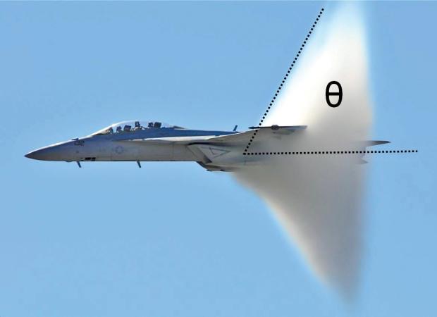
Geometrically, the shock front forms a cone around the object, which under certain circumstances can even be visible to the naked eye (see image below). The great formula that is featured in this section deals with the opening angle of said cone. This angle, symbolized by the Greek letter θ, is also indicated in the image.

All we need to compute the mach angle θ is the velocity of the object v (in m/s) and speed of sound c (in m/s):

sin θ = c / v

Let’s turn to an example.

———————-

A jet fighter flies with a speed of v = 500 m/s toward its destination. It flies close to the ground, so the speed of sound is approximately c = 340 m/s. This leads to:

sin θ = 340 / 500 = 0.68

θ = arcsin(0.68) ≈ 43°

———————-

In the picture above the angle is approximately 62°. How fast was the jet going at the time when the picture was taken? We’ll set the speed of sound to c = 340 m/s and insert all the given data into the formula:

sin 62° = 340 / v

0.88 = 340 / v

Obviously we need to solve for v. To do that, we first multiply both sides by v. This leads to:

0.88 · v = 340

Dividing both sides by 0.88 results in the answer:

v = 340 / 0.88 ≈ 385 m/s ≈ 1390 km/h ≈ 860 mph

———————-

This was an excerpt from the ebook “Great Formulas Explained – Physics, Mathematics, Economics”, released yesterday and available here: http://www.amazon.com/dp/B00G807Y00.

The Time Value of Money and Inflation

To make a point, I’ll start this blog entry in an unusual way, that is, by talking about vectors. A vector is basically an ordered row of numbers. Consider this expression for example:

(12, 3, 5)

This vector could represent a lot of things. For example a point in a three dimensional coordinate system, with the vector components being the x-, y- and z-values respectively. Or for a company offering three products, it could stand for the sales of these products in a certain year.

Why this talk about vectors? You were probably very surprised when you heard grandma say that she paid only 150 $ for her first car. It seems so amazingly cheap. But it is not. Your dear grandma is talking about 1950’s money, while you are thinking of today’s money. These two have a very different value.

If you want to specify the costs of a good precisely, merely giving an amount of money will not be sufficient. The value of money changes over time and thus to be absolutely precise, you should always couple this amount with a certain year. For example, this is what grandma’s car really cost:

(150 $, 1950)

This is far from (150 $, 2012), which is what you were thinking of when grandma shared the story with you. Using an online inflation calculator, we can conclude that this is actually what the car would cost in today’s money:

(1410 $, 2012)

Not an expensive car, but certainly more than 150 $ in today’s money. Now you can see why I started this chapter using vectors. They allow us to easily and clearly couple an amount with a year. A true pedant would even ask for one more component since we are still missing the respective months. But let’s not get too pedantic.

How can we justify saying that 150 $ in 1950’s money is the same as 1410 $ in today’s money? We can look at how much of a certain good these amounts would buy in the given year. With 150 $ in 1950 you could fill your basket with about as many apples as you can with 1410 $ today. The same goes for most other common goods: oranges, potatoes, water, cinema tickets, and so on.

This is inflation, goods get more expensive each year. At a later point we will take a look at what reasons there are for inflation to occur. But before that, let’s define the rate of inflation and see how it is measured …

This was an excerpt from the ebook “Business Math Basics – Practical and Simple”, available for Kindle here: http://www.amazon.com/dp/B00FXB8QSO.

Probability and Multiple Choice Tests

Imagine taking a multiple choice test that has three possible answers to each question. This means that even if you don’t know any answer, your chance of getting a question right is still 1/3. How likely is it to get all questions right by guessing if the test contains ten questions?

Here we are looking at the event “correct answer” which occurs with a probability of p(correct answer) = 1/3. We want to know the odds of this event happening ten times in a row. For that we simply apply the multiplication rule:

• p(all correct) = (1/3)¹⁰ = 0.000017

Doing the inverse, we can see that this corresponds to about 1 in 60000. So if we gave this test to 60000 students who only guessed the answers, we could expect only one to be that lucky. What about the other extreme? How likely is it to get none of the ten questions right when guessing?

Now we must focus on the event “incorrect answer” which has the probability p(incorrect answer) = 2/3. The odds for this to occur ten times in a row is:

• p(all incorrect) = (2/3)¹⁰ = 0.017

In other words: 1 in 60. Among the 60000 guessing students, this outcome can be expected to appear 1000 times. How would these numbers change if we only had eight instead of ten questions? Or if we had four options per question instead of three? I leave this calculation up to you.

Physics (And The Formula That Got Me Hooked)

A long time ago, in my teen years, this was the formula that got me hooked on physics. Why? I can’t say for sure. I guess I was very surprised that you could calculate something like this so easily. So with some nostalgia, I present another great formula from the field of physics. It will be a continuation of and a last section on energy.

To heat something, you need a certain amount of energy E (in J). How much exactly? To compute this we require three inputs: the mass m (in kg) of the object we want to heat, the temperature difference T (in °C) between initial and final state and the so called specific heat c (in J per kg °C) of the material that is heated. The relationship is quite simple:

E = c · m · T

If you double any of the input quantities, the energy required for heating will double as well. A very helpful addition to problems involving heating is this formula:

E = P · t

with P (in watt = W = J/s) being the power of the device that delivers heat and t (in s) the duration of the heat delivery.

———————

The specific heat of water is c = 4200 J per kg °C. How much energy do you need to heat m = 1 kg of water from room temperature (20 °C) to its boiling point (100 °C)? Note that the temperature difference between initial and final state is T = 80 °C. So we have all the quantities we need.

E = 4200 · 1 · 80 = 336,000 J

Additional question: How long will it take a water heater with an output of 2000 W to accomplish this? Let’s set up an equation for this using the second formula:

336,000 = 2000 · t

t ≈ 168 s ≈ 3 minutes

———————-

We put m = 1 kg of water (c = 4200 J per kg °C) in one container and m = 1 kg of sand (c = 290 J per kg °C) in another next to it. This will serve as an artificial beach. Using a heater we add 10,000 J of heat to each container. By what temperature will the water and the sand be raised?

Let’s turn to the water. From the given data and the great formula we can set up this equation:

10,000 = 4200 · 1 · T

T ≈ 2.4 °C

So the water temperature will be raised by 2.4 °C. What about the sand? It also receives 10,000 J.

10,000 = 290 · 1 · T

T ≈ 34.5 °C

So sand (or any ground in general) will heat up much stronger than water. In other words: the temperature of ground reacts quite strongly to changes in energy input while water is rather sluggish. This explains why the climate near oceans is milder than inland, that is, why the summers are less hot and the winters less cold. The water efficiently dampens the changes in temperature.

It also explains the land-sea-breeze phenomenon (seen in the image below). During the day, the sun’s energy will cause the ground to be hotter than the water. The air above the ground rises, leading to cooler air flowing from the ocean to the land. At night, due to the lack of the sun’s power, the situation reverses. The ground cools off quickly and now it’s the air above the water that rises.

———————-

I hope this formula got you hooked as well. It’s simple, useful and can explain quite a lot of physics at the same time. It doesn’t get any better than this. Now it’s time to leave the concept of energy and turn to other topics.

This was an excerpt from my Kindle ebook: Great Formulas Explained – Physics, Mathematics, Economics. For another interesting physics quicky, check out: Intensity (or: How Much Power Will Burst Your Eardrums?).

Physics: Free Fall and Terminal Velocity

After a while of free fall, any object will reach and maintain a terminal velocity. To calculate it, we need a lot of inputs.

The necessary quantities are: the mass of the object (in kg), the gravitational acceleration (in m/s²), the density of air D (in kg/m³), the projected area of the object A (in m²) and the drag coefficient c (dimensionless). The latter two quantities need some explaining.

The projected area is the largest cross-section in the direction of fall. You can think of it as the shadow of the object on the ground when the sun’s rays hit the ground at a ninety degree angle. For example, if the falling object is a sphere, the projected area will be a circle with the same radius.

The drag coefficient is a dimensionless number that depends in a very complex way on the geometry of the object. There’s no simple way to compute it, usually it is determined in a wind tunnel. However, you can find the drag coefficients for common shapes in the picture below.

Now that we know all the inputs, let’s look at the formula for the terminal velocity v (in m/s). It will be valid for objects dropped from such a great heights that they manage to reach this limiting value, which is basically a result of the air resistance canceling out gravity.

v = sq root (2 * m * g / (c * D * A) )

Let’s do an example.

Skydivers are in free fall after leaving the plane, but soon reach the terminal velocity. We will set the mass to m = 75 kg, g = 9.81 (as usual) and D = 1.2 kg/m³. In a head-first position the skydiver has a drag coefficient of c = 0.8 and a projected area A = 0.3 m². What is the terminal velocity of the skydiver?

v = sq root (2 * 75 * 9.81 / (0.8 * 1.2 * 0.3) )

v ≈ 70 m/s ≈ 260 km/h ≈ 160 mph

Let’s take a look how changing the inputs varies the terminal velocity. Two bullet points will be sufficient here:

• If you quadruple the mass (or the gravitational acceleration), the terminal velocity doubles. So a very heavy skydiver or a regular skydiver on a massive planet would fall much faster.

• If you quadruple the drag coefficient (or the density or the projected area), the terminal velocity halves. This is why parachutes work. They have a higher drag coefficient and larger area, thus effectively reducing the terminal velocity.

This was an excerpt from the Kindle ebook: Great Formulas Explained – Physics. Mathematics, Economics. Check out my BEST OF for more interesting physics articles.

How much habitable land is there on earth per person?

What is the total area of habitable land on Earth? And how much habitable land does that leave one person? We’ll use the value r = 6400 km as the radius of Earth. According to the corresponding formula for spheres, the surface area of Earth is:

S = 4 * π * (6400 km)^2 ≈ 515 million square km

Since about 30 % of Earth’s surface is land, this means that the total area of land is 0.3 * 515 ≈ 155 million square km, about half of which is habitable for humans. With roughly 7 billion people alive today, we can conclude that there is 0.011 square km habitable land available per person. This corresponds to a square with 100 m ≈ 330 ft length and width.

More Pirates, Less Global Warming … wait, what?

An interesting correlation was found by the parody religion FSM (Flying Spaghetti Monster). Deducting causation here would be madness. Over the 18th and 19th century, piracy, the one with the boats, not the one with the files and the sharing, slowly died out. At the same time, possibly within a natural trend and / or for reasons of increased industrial activity, the global temperature started increasing. If you plot the number of pirates and the global temperature in a coordinate system, you find a relatively strong correlation between the two. The more pirates there are, the colder the planet is. Here’s the corresponding formula and graph:

 T = 16 – 0.05 · P^0.33

 

with T being the average global temperature and P the number of pirates. Given enough pirates (about 3.3 million to be specific), we could even freeze Earth. But of course nobody in the right mind would see causality at work here, rather we have two processes, the disappearance of piracy and global warming, that happened to occur at the same time. So you shouldn’t be too surprised that the recent rise of piracy in Somalia didn’t do anything to stop global warming.

A tunnel through earth and a surprising result …

Recently I found an interesting problem: A straight tunnel is being drilled through the earth (see picture; tunnel is drawn with two lines) and rails are installed in the tunnel. A train travels, only driven by gravitation and frictionless, along the rails. How long does it take the train to travel through this earth tunnel of length l?

The calculation, shows a surprising result. The travel time is independent of the length l; the time it takes the train to travel through a 1 Km tunnel is the same as through a 5000 Km tunnel, about 2500 seconds or 42 minutes! Why is that?

Imagine a model train on rails. If you put the rails on flat ground, the train won’t move. The gravitational force is pulling on the train, but not in the direction of travel. If you incline the rails slighty, the train starts to move slowly, if you incline the rails strongly, it rapidly picks up speed.

Now lets imagine a tunnel through the earth! A 1 Km tunnel will only have a slight inclination and the train would accelerate slowly. It would be a pleasant trip for the entire family. But a 5000 Km train would go steeply into the ground, the train would accelerate with an amazing rate. It would be a hell of a ride! This explains how we always get the same travel time: the 1 Km tunnel is short and the velocity would remain low, the 5000 Km is long, but the velocity would become enormous.

Here is how the hell ride through the 5000 Km tunnel looks in detail:

The red, monotonous increasing curve, shows distance traveled (in Km) versus time (in seconds), the blue curve shows velocity (in Km/s) versus time. In the center of the tunnel the train reaches the maximum velocity of about 3 Km/s, which corresponds to an incredible 6700 mi/h!

Statistics and Monkeys on Typewriters

Here are the first two sentences of the prologue to Shakespeare’s Romeo and Juliet:

Two households, both alike in dignity,
In fair Verona, where we lay our scene

This excerpt has 77 characters. Now we let a monkey start typing random letters on a typewriter. Once he typed 77 characters, we change the sheet and let him start over. How many tries does he need to randomly reproduce the above paragraph?

There are 26 letters in the English alphabet and since he’ll be needing the comma and space, we’ll include those as well. So there’s a 1/28 chance of getting the first character right. Same goes for the second character, third character, etc … Because he’s typing randomly, the chance of getting a character right is independent of what preceded it. So we can just start multiplying:

p(reproduce) = 1/28 · 1/28 · … · 1/28 = (1/28)^77

The result is about 4 times ten to the power of -112. This is a ridiculously small chance! Even if he was able to complete one quadrillion tries per millisecond, it would most likely take him considerably longer than the estimated age of the universe to reproduce these two sentences.

Now what about the first word? It has only three letters, so he should be able to get at least this part in a short time. The chance of randomly reproducing the word “two” is:

p(reproduce) = 1/26 · 1/26 · 1/26 = (1/26)^3

Note that I dropped the comma and space as a choice, so now there’s a 1 in 26 chance to get a character right. The result is 5.7 times ten to the power of -5, which is about a 1 in 17500 chance. Even a slower monkey could easily get that done within a year, but I guess it’s still best to stick to human writers.

.This was an excerpt from the ebook “Statistical Snacks. Liked the excerpt? Get the book here: http://www.amazon.com/Statistical-Snacks-ebook/dp/B00DWJZ9Z2. Want more excerpts? Check out The Probability of Becoming a Homicide Victim and Missile Accuracy (CEP).

From Simple to Compound Interest

Imagine you loan a bank the principal P = 10000 $ at an interest rate of i = 5 %. This is the amount of interest you would receive with simple interest, given the duration t of the loan:

t = 1 year
→ I = 10000 $ * 0.05 * 1 = 500 $

t = 2 years
→ I = 10000 $ * 0.05 * 2 = 1000 $

t = 3 years
→ I = 10000 $ * 0.05 * 3 = 1500 $

As you can see, the interest grows linearly with the duration of the loan. For each additional year, you get an additional 500 $, which is just 5 % of the principal 10000 $. In other words: each year the interest rate is applied to the principal. How could that be any different?

Consider this: At the end of the first year, you’ll receive an interest payment in the amount of 500 $. This means that your bank statement will now read 10000 $ + 500 $  = 10500 $. So why not apply the interest rate to this updated value? This would lead to an interest payment of 10500 $ * 0.05 = 525 $ for the second year instead of just 500 $.

Continuing this train of thought, at the end of the second year your bank statement would read 10000 $ + 500 $ + 525 $ = 11025 $. Again we would rather have the interest rate applied to this updated value instead of the unchanging principal. This would result in an interest payment of 11025 $ * 0.05 = 551.25 $ for the third year.

For comparison, here’s what the final pay out would be for the simple interest plan:

10000 $ + 500 $ + 500 $ + 500 $ = 11500 $

And this is what we would get with the “not simple” interest plan, where we apply the interest rate to the updated amounts instead of the principal:

10000 $ + 500 $ + 525 $ + 551.25 $ = 11576.25 $

The latter is called compound interest. It means that we include already paid interests in the calculation of next year’s interest, which leads to the amount received growing exponentially instead of linearly.

(This was an excerpt from “Business Math Basics – Practical and Simple”. You can get it here: http://www.amazon.com/Business-Math-Basics-Practical-Simple-ebook/dp/B00FXB8QSO/)

Average Size of Web Pages plus Prediction

Using data from websiteoptimization.com I plotted the development of web page sizes over the years. I also included the exponential fit:

As you can see, the 1/2 MB mark was cracked in 2009 and the 1 MB mark was cracked in 2012. Despite the seemingly random fluctuations, an exponential trend is clearly visible. The power 0.3 indicates that the web page sizes doubles about every 2.3 years. Assuming this exponential trend continues we will have these average sizes in the coming years:

2013 – ca. 1600 kb
2014 – ca. 2100 kb
2015 – ca. 2900 kb

So the 2 MB will probably be cracked in 2014 and in 2015 we will already be close to the 3 MB mark. Of course the trend is bound to flat out, but at this point there’s no telling when it will happen.

If you like more Internet analysis, check out The Internet since 1998 in Numbers.

Missile Accuracy (CEP) – Excerpt from “Statistical Snacks”

An important quantity when comparing missiles is the CEP (Circular Error Probable). It is defined as the radius of the circle in which 50 % of the fired missiles land. The smaller it is, the better the accuracy of the missile. The German V2 rockets for example had a CEP of about 17 km. So there was a 50/50 chance of a V2 landing within 17 km of its target. Targeting smaller cities or even complexes was next to impossible with this accuracy, one could only aim for a general area in which it would land rather randomly.

Today’s missiles are significantly more accurate. The latest version of China’s DF-21 has a CEP about 40 m, allowing the accurate targeting of small complexes or large buildings, while CEP of the American made Hellfire is as low as 4 m, enabling precision strikes on small buildings or even tanks.

Assuming the impacts are normally distributed, one can derive a formula for the probability of striking a circular target of Radius R using a missile with a given CEP:

p = 1 – exp( -0.41 · R² / CEP² )

This quantity is also called the “single shot kill probability” (SSKP). Let’s include some numerical values. Assume a small complex with the dimensions 100 m by 100 m is targeted with a missile having a CEP of 150 m. Converting the rectangular area into a circle of equal area gives us a radius of about 56 m. Thus the SSKP is:

p = 1 – exp( -0.41 · 56² / 150² ) = 0.056 = 5.6 %

So the chances of hitting the target are relatively low. But the lack in accuracy can be compensated by firing several missiles in succession. What is the chance of at least one missile hitting the target if ten missiles are fired? First we look at the odds of all missiles missing the target and answer the question from that. One missile misses with 0.944 probability, the chance of having this event occur ten times in a row is:

p(all miss) = 0.944¹⁰ = 0.562

Thus the chance of at least one hit is:

p(at least one hit) = 1 – 0.562 = 0.438 = 43.8 %

Still not great considering that a single missile easily costs 10000 $ upwards. How many missiles of this kind must be fired at the complex to have a 90 % chance at a hit? A 90 % chance at a hit means that the chance of all missiles missing is 10 %. So we can turn the above formula for p(all miss) into an equation by inserting p(all miss) = 0.1 and leaving the number of missiles n undetermined:

0.1 = 0.944ⁿ

All that’s left is doing the algebra. Applying the natural logarithm to both sides and solving for n results in:

n = ln(0.1) / ln(0.944) = 40

So forty missiles with a CEP of 150 m are required to have a 90 % chance at hitting the complex. As you can verify by doing the appropriate calculations, three DF-21 missiles would have achieved the same result.

Liked the excerpt? Get the book “Statistical Snacks” by Metin Bektas here: http://www.amazon.com/Statistical-Snacks-ebook/dp/B00DWJZ9Z2. For more excerpts see The Probability of Becoming a Homicide Victim and How To Use the Expected Value.

My Fair Game – How To Use the Expected Value

You meet a nice man on the street offering you a game of dice. For a wager of just 2 $, you can win 8 $ when the dice shows a six. Sounds good? Let’s say you join in and play 30 rounds. What will be your expected balance after that?

You roll a six with the probability p = 1/6. So of the 30 rounds, you can expect to win 1/6 · 30 = 5, resulting in a pay-out of 40 $. But winning 5 rounds of course also means that you lost the remaining 25 rounds, resulting in a loss of 50 $. Your expected balance after 30 rounds is thus -10 $. Or in other words: for the player this game results in a loss of 1/3 $ per round.

 Let’s make a general formula for just this case. We are offered a game which we win with a probability of p. The pay-out in case of victory is P, the wager is W. We play this game for a number of n rounds.

The expected number of wins is p·n, so the total pay-out will be: p·n·P. The expected number of losses is (1-p)·n, so we will most likely lose this amount of money: (1-p)·n·W.

 Now we can set up the formula for the balance. We simply subtract the losses from the pay-out. But while we’re at it, let’s divide both sides by n to get the balance per round. It already includes all the information we need and requires one less variable.

B = p · P – (1-p) · W

This is what we can expect to win (or lose) per round. Let’s check it by using the above example. We had the winning chance p = 1/6, the pay-out P = 8 $ and the wager W = 2 $. So from the formula we get this balance per round:

B = 1/6 · 8 $ – 5/6 · 2 $ = – 1/3 $ per round

Just as we expected. Let’s try another example. I’ll offer you a dice game. If you roll two six in a row, you get P = 175 $. The wager is W = 5 $. Quite the deal, isn’t it? Let’s see. Rolling two six in a row occurs with a probability of p = 1/36. So the expected balance per round is:

B = 1/36 · 175 $ – 35/36 · 5 $ = 0 $ per round

I offered you a truly fair game. No one can be expected to lose in the long run. Of course if we only play a few rounds, somebody will win and somebody will lose.

It’s helpful to understand this balance as being sound for a large number of rounds but rather fragile in case of playing only a few rounds. Casinos are host to thousands of rounds per day and thus can predict their gains quite accurately from the balance per round. After a lot of rounds, all the random streaks and significant one-time events hardly impact the total balance anymore. The real balance will converge to the theoretical balance more and more as the number of rounds grows. This is mathematically proven by the Law of Large Numbers. Assuming finite variance, the proof can be done elegantly using Chebyshev’s Inequality.

The convergence can be easily demonstrated using a computer simulation. We will let the computer, equipped with random numbers, run our dice game for 2000 rounds. After each round the computer calculates the balance per round so far. The below picture shows the difference between the simulated balance per round and our theoretical result of – 1/3 $ per round.

(Liked the excerpt? Get the book “Statistical Snacks” by Metin Bektas here: http://www.amazon.com/Statistical-Snacks-ebook/dp/B00DWJZ9Z2)